GLM 2: Categorical Predictors

Princeton University

Jason Geller, PH.D.(he/him)

2023-10-23

Announcements

Final paper plan is due next week
Keanan Joyner is giving a talk tomorrow (12:00 P.M.)
- No workshop

Packages

library(grateful)
pkgs <- cite_packages(output = "table", out.dir = ".")

pkgs

       Package  Version                                       Citation
1         afex    1.1.1                                          @afex
2         base    4.2.2                                          @base
3    easystats  0.6.0.8                                     @easystats
4      emmeans    1.8.0                                       @emmeans
5         faux    1.1.0                                          @faux
6           gt    0.8.0                                            @gt
7         here    1.0.1                                          @here
8   kableExtra    1.3.4                                    @kableExtra
9        knitr     1.41             @knitr2014; @knitr2015; @knitr2022
10  modelbased  0.8.6.3                                    @modelbased
11      pacman    0.5.1                                        @pacman
12  parameters 0.21.1.2                                    @parameters
13 performance 0.10.4.1                                   @performance
14   rmarkdown     2.14 @rmarkdown2018; @rmarkdown2020; @rmarkdown2022
15   supernova    2.5.6                                     @supernova
16   tidyverse    1.3.2                                     @tidyverse
17     ungeviz    0.1.0                                       @ungeviz

Follow Along

https://github.com/jgeller112/PSY503-F2023/blob/main/slides/09-Cat-Reg/09-Cat-Pred.qmd

Today

How to interpret linear models with categorical predictors
- Two or more levels
Explain the different ways to break down categorical predictors in linear models
- Dummy coding
- Sum Coding
- Deviation coding
- DIY/custom contrasts

Multiple comparisons
Plotting

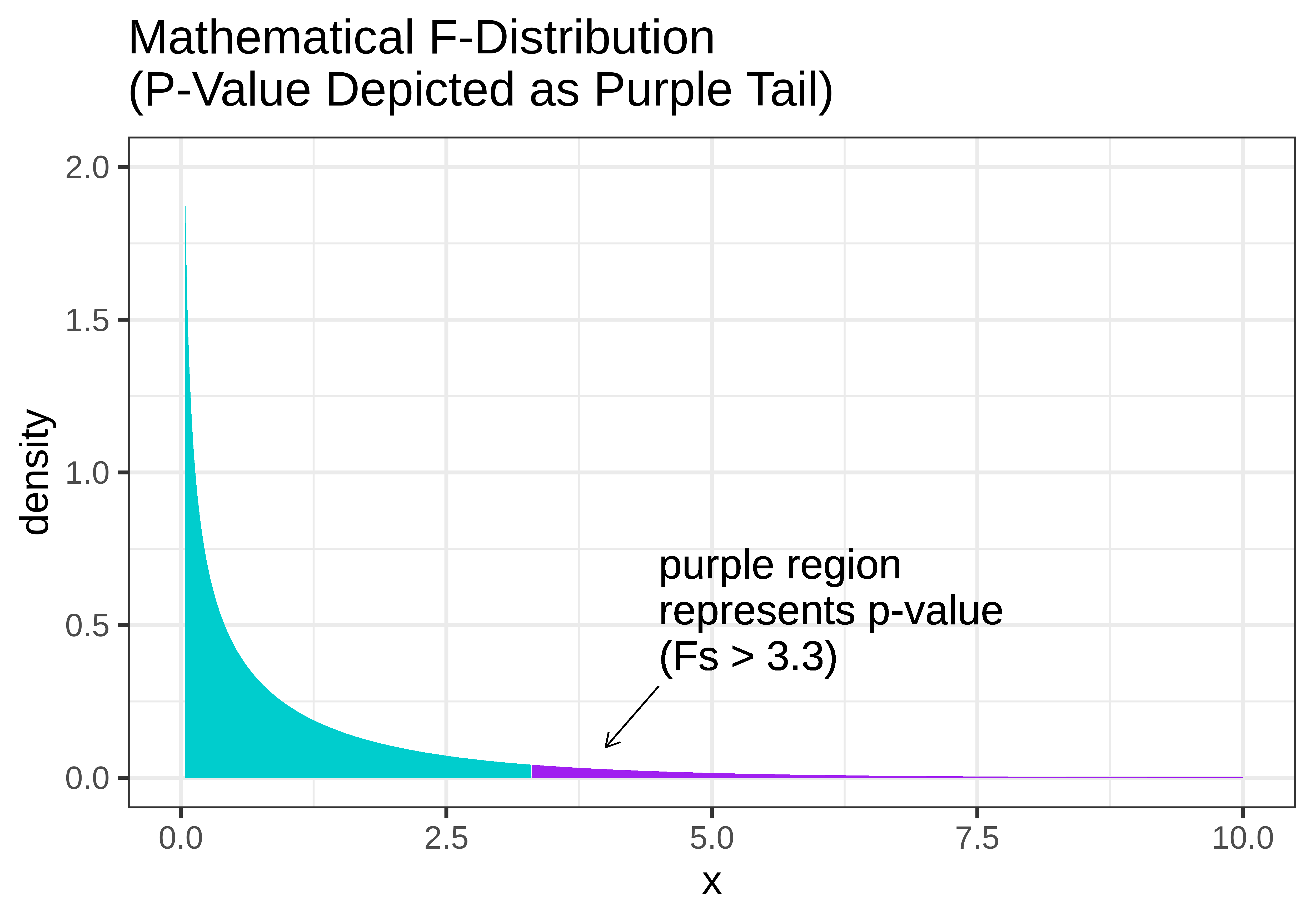
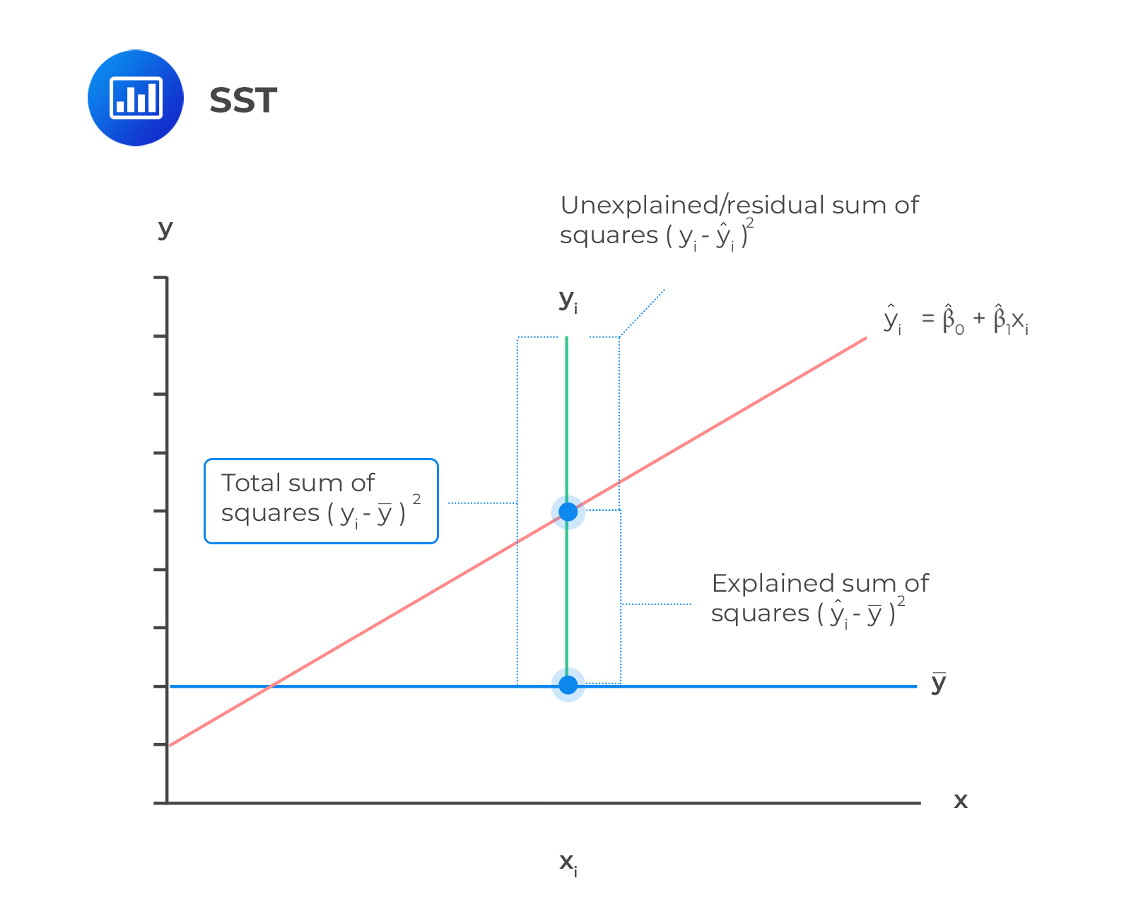
F-Distribution/F-test

\[F = \frac{SS_{Explained}/df1 (p-1)}{SS_{Unexplained}/df2(n-p)} = \frac{MS_{Explained}}{MS_{Unexplained}}\]

MS explained represents the reduction in error achieved by the model
MS unexplained tells us how much variation is left over from the complex model

Modeling Categorical Variables

Today’s dataset
- Winter(2016)
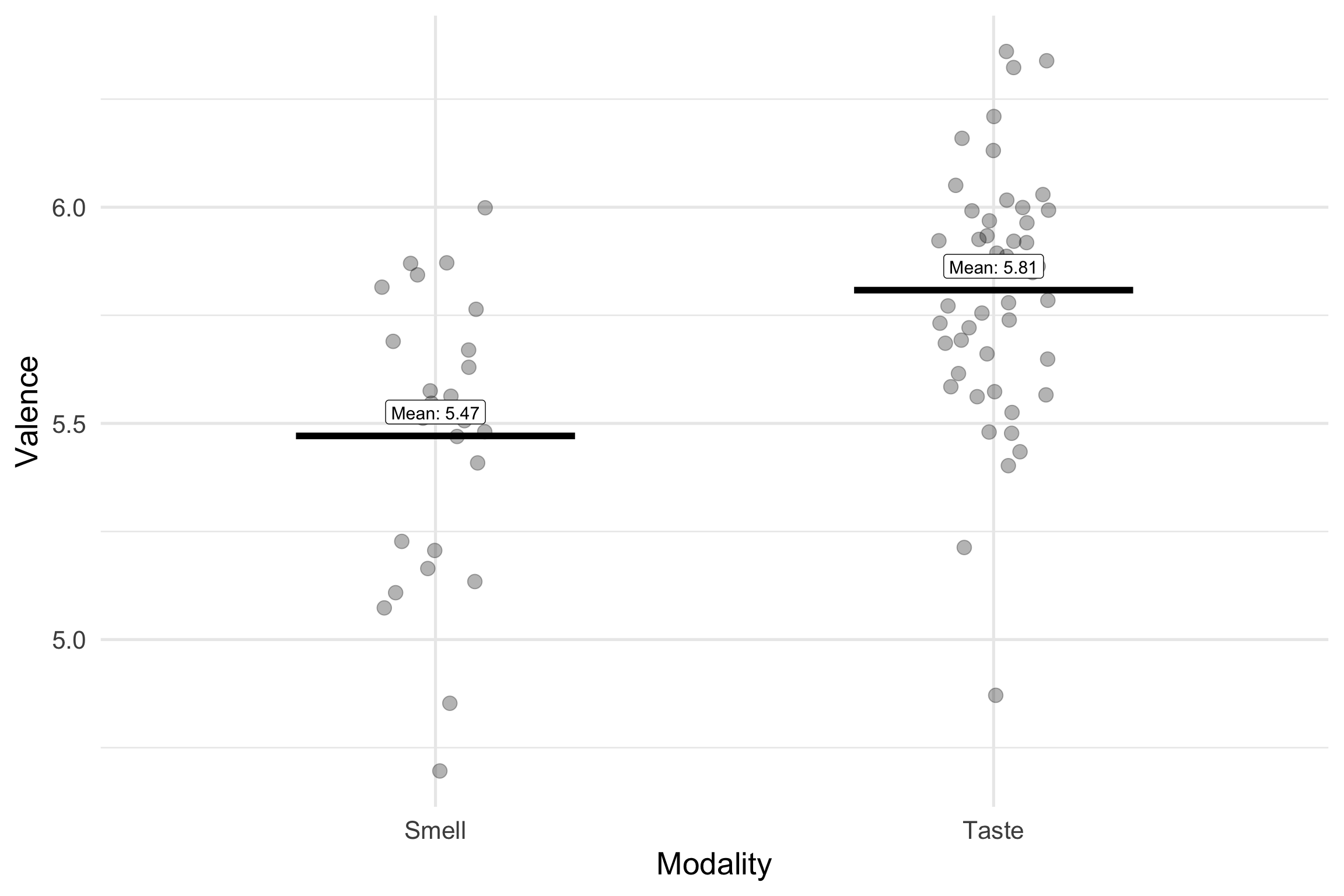
  - Are smell words (e.g., rancid) rated as more negative/unpleasant than taste words (e.g., sweet)?
    - 1 to 9 rating scale

senses<- read_csv(here::here("slides/09-Cat-Reg/data/winter_2016_senses_valence.csv"))

senses_filt <- senses %>%
  filter(Modality=="Taste" | Modality=="Smell")

glimpse(senses_filt)

Rows: 72
Columns: 3
$ Word     <chr> "acidic", "acrid", "alcoholic", "antiseptic", "aromatic", "as…
$ Modality <chr> "Taste", "Smell", "Taste", "Smell", "Smell", "Taste", "Taste"…
$ Val      <dbl> 5.539592, 5.173947, 5.557228, 5.511795, 5.952941, 5.965000, 6…

Linear Model

\[{Y_i} = b_0 + b_1 {X_i} + e\]

So far predictor variable has been continuous
We can also use linear modeling for categorical variables!

Categorical Variables

Terminology
- Factor: a variable with a fix set of categories
- Levels: The individual categories within a factor
In our dataset, what is the factor and what are its levels?

is.factor(senses_filt$Modality)

[1] FALSE

senses_filt %>% 
  mutate(Modality=factor(Modality), 
         Modality=as.factor(Modality))

# A tibble: 72 × 3
   Word       Modality   Val
   <chr>      <fct>    <dbl>
 1 acidic     Taste     5.54
 2 acrid      Smell     5.17
 3 alcoholic  Taste     5.56
 4 antiseptic Smell     5.51
 5 aromatic   Smell     5.95
 6 astringent Taste     5.96
 7 barbecued  Taste     6.05
 8 beery      Taste     6.07
 9 bitter     Taste     5.12
10 bland      Taste     5.75
# ℹ 62 more rows

Important

Always make sure categorical variables are labeled as factors in your dataset

Linear Modeling and t-tests/ANOVAs

What do we do in linear modeling?

Fit a line (least squares method)

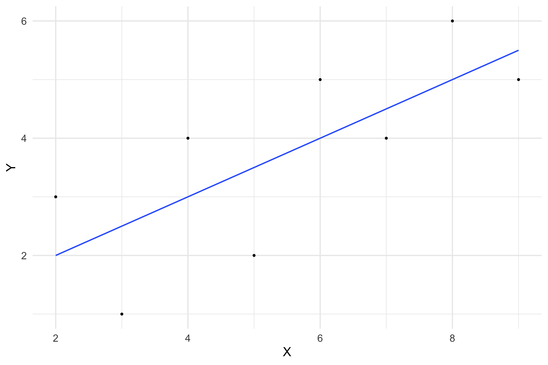
Linear Modeling and t-tests/ANOVAs

Within a t-test/ANOVA framework we want to know if means differ between groups

Fit a line

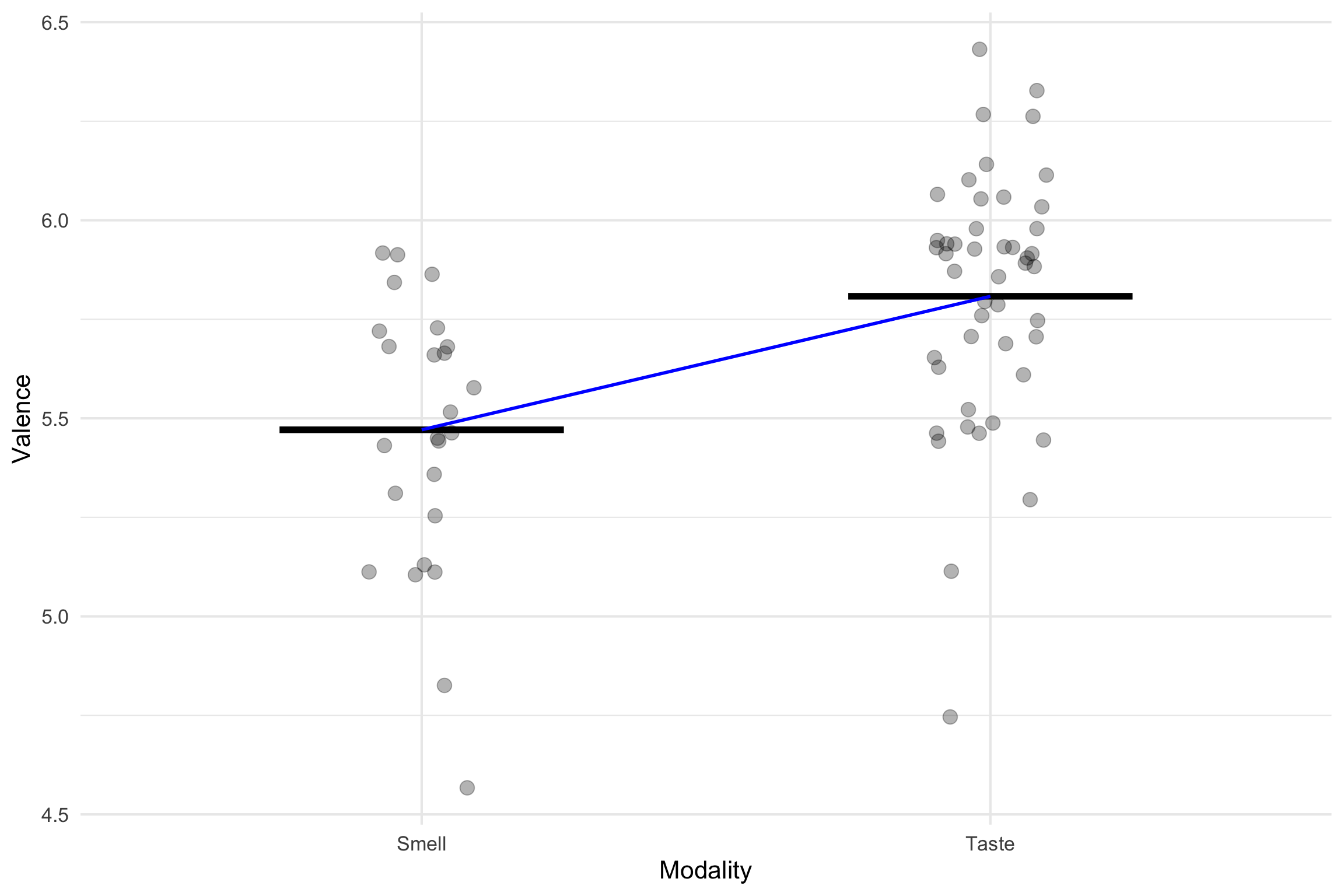
Single Line

We have two equations
- \(y = b_0\) = intercept(mean of smell)
- \(y = b_0\) = intercept(mean of touch)
How do we get one linear equation?

Dummy Coding/Treatment Coding

R’s default system
- Start with \(K\) levels
- Break variable into \(K\)-1 dummy variables, which are coded as 0 and 1
  - Variable coded as 0 is with reference level
    - R does this automatically (0 = whatever comes first alphabetically)
      - Smell = 0
      - Taste = 1

Dummy Coding/Treatment Coding

\[\operatorname{Valence} = b_0 + b_{1}(X_i) + \epsilon\]

Prediction for Smell \(X_i =0\)

\[\hat{\operatorname{Val}} = b_0 + b_{1}(\operatorname{Modality}_{\operatorname{Taste}}0) + \epsilon\] \[ \operatorname{\bar{Y}_{smell}} = b_0 \]

Prediction for Taste \(X_i =1\)

\[\operatorname{Val} = b_0 + b_{1}(\operatorname{Modality}_{\operatorname{Taste}}1) + \epsilon\] \[\operatorname{\bar{Y}_{taste}} = b_0 + b_1(\operatorname{Modality}_{\operatorname{Taste}}1)\]

Dummy coding

## dummy coding
senses_dum <- senses_filt %>%
  mutate(mod=ifelse(Modality=="Smell", 0, 1))


senses_dum

# A tibble: 72 × 4
   Word       Modality   Val   mod
   <chr>      <chr>    <dbl> <dbl>
 1 acidic     Taste     5.54     1
 2 acrid      Smell     5.17     0
 3 alcoholic  Taste     5.56     1
 4 antiseptic Smell     5.51     0
 5 aromatic   Smell     5.95     0
 6 astringent Taste     5.96     1
 7 barbecued  Taste     6.05     1
 8 beery      Taste     6.07     1
 9 bitter     Taste     5.12     1
10 bland      Taste     5.75     1
# ℹ 62 more rows

Dummy coded regression

lm_treat <- lm(Val ~ mod, data=senses_dum)

term	estimate	std.error	statistic	p.value	conf.low	conf.high
(Intercept)	5.4710116	0.0629655	86.889060	0.00e+00	5.3454309	5.5965923
mod	0.3371123	0.0779327	4.325684	4.95e-05	0.1816804	0.4925442

\(\hat{b_0}\): The mean of smell (5.47). When X = 0 (Smell), y = 5.47
\(\hat{b_1}\):

Categorical contrast coding

\[slope=\frac{\mu_{diff}}{run}\]

Dummy Coded Regression

term	estimate	std.error	statistic	p.value	conf.low	conf.high
(Intercept)	5.4710116	0.0629655	86.889060	0.00e+00	5.3454309	5.5965923
mod	0.3371123	0.0779327	4.325684	4.95e-05	0.1816804	0.4925442

\(\hat{b_1}\): The mean difference between the two groups. If you go from one category to another, there is a .337 difference between the two groups

Calculate Means

Let’s calculate the means for each group with this equation

# mean of smell

#b_0 + b_1(0)
5.47 + (.337)*(0)

[1] 5.47

#b_0 + b_1(1)
# mean of taste
5.47 + (.337)*1

[1] 5.807

Change Reference Level

senses_dum <- senses_filt %>%
  mutate(mod=factor(Modality)) %>% 
  mutate(mod1=relevel(mod, ref="Taste"))
#relevel the var 
#contrasts(senses_dum$mod1)
#contrasts(senses_dum$mod)

term	estimate	std.error	statistic	p.value	conf.low	conf.high
(Intercept)	5.8081239	0.0459223	126.477205	0.00e+00	5.7165348	5.8997130
mod1Smell	-0.3371123	0.0779327	-4.325684	4.95e-05	-0.4925442	-0.1816804

Contrast coding/Sum-to-zero

Deviation coding/sum coding

So far the intercept at 0 has referred to a particular baseline or reference level
Sum-to-zero coding changes the intercept to correspond to mean of the means (grand mean)

\[\frac{\mu_1 + \mu_2}{2}\]

Note

When sample sizes for each group are equal the grand mean and mean of means will be equal

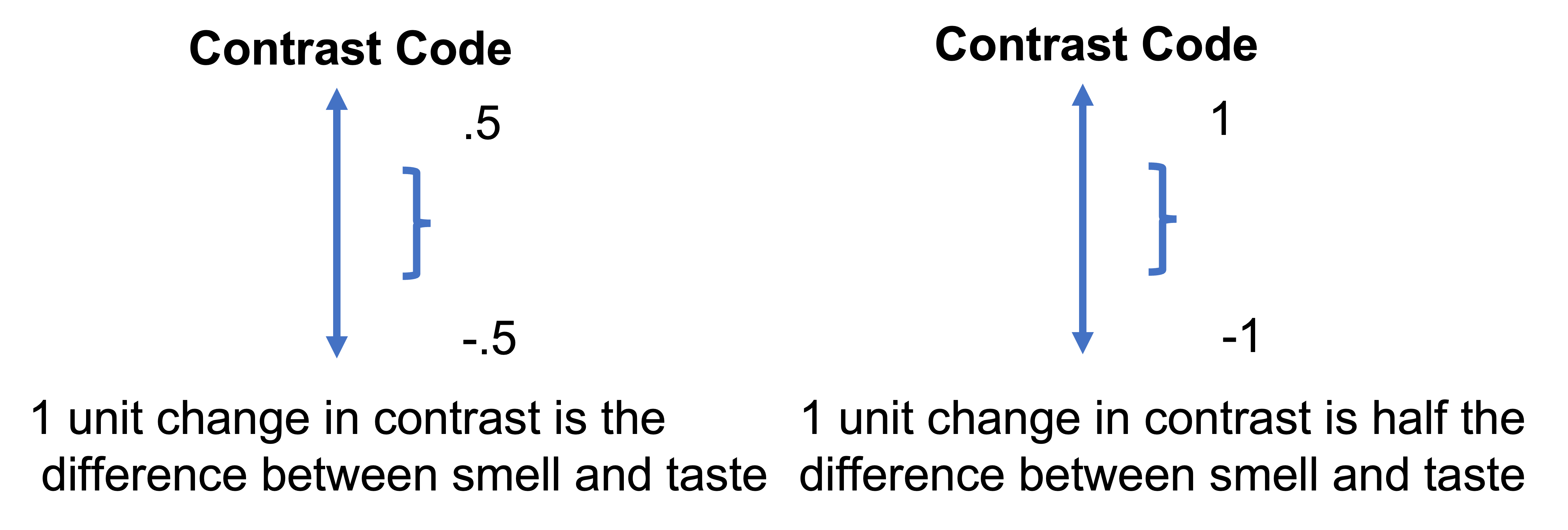
Deviation coding (.5, -.5)

Note

Lot’s of confusion over terms. I will be using Lisa Debruine’s definitions https://debruine.github.io/faux/articles/contrasts.html

\(\hat{b_0}\) (intercept) is now the grand mean
Slope is still the difference

Deviation coding

# how do apply deviation code
senses_filt_dev <- senses_filt %>%
  mutate(mod_dev=as.factor(Modality)) %>%
  #man code it
  mutate(modo_dev=ifelse(Modality=="Smell", .5, -.5))
  #add a new var to dev code 

contrasts(senses_filt_dev$mod_dev) <- c(0.5, -0.5) # change 0 - 1 to +.5 and -.5

Deviation Coding Results

lm_dev <- lm(Val ~ mod_dev, data=senses_filt_dev)

term	estimate	std.error	statistic	p.value	conf.low	conf.high
(Intercept)	5.6395677	0.0389664	144.729132	0.00e+00	5.5618518	5.7172837
mod_dev1	-0.3371123	0.0779327	-4.325684	4.95e-05	-0.4925442	-0.1816804

\(\hat{b_0}\): The value of the intercept is the mean of the means (5.64)
\(\hat{b_1}\): The difference between Smell and taste
\(\bar{Y}_{smell} = b_0 + b_1(.5)\)
\(\bar{Y}_{taste}: b_0 + b_1(-.5)\)

Sum Coding

1 and -1

senses_filt_sum <- senses_filt_dev %>%
  mutate(mod_sum55=ifelse(mod_dev=="Taste", .5, -.5), 
mod_sum11 = ifelse(mod_dev=="Smell", 1, -1)) # add a new var to sum code (1, -1)


contrasts(senses_filt_sum$mod_dev) <- c(1, -1)

Sum Coding (-1 + 1) Interpretation

What does this do to our interpretation?

Intercept is still centered at 0 (grand mean)
Slope is still the same (difference between categories) but:
- Stepping from one category to another (the run) results in overall change of 2
- Results are halved

Sum Coding (-1 + 1) Interpretation

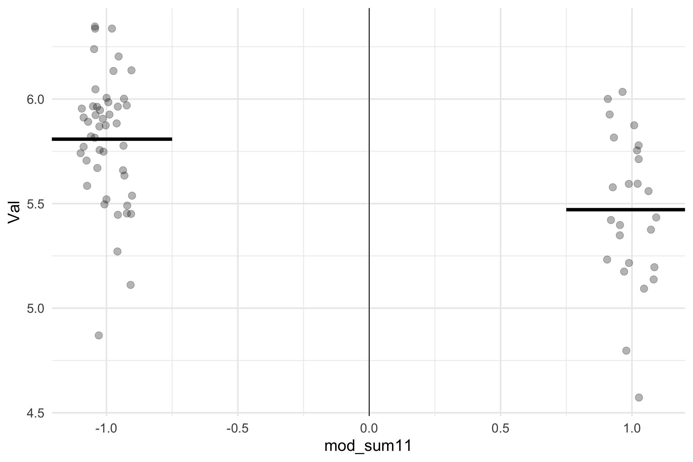
Sum Coding (+1, -1) Model Results

lm_sum <- lm(Val ~ mod_sum11, data=senses_filt_sum)

term	estimate	std.error	statistic	p.value	conf.low	conf.high
(Intercept)	5.6395677	0.0389664	144.729132	0.00e+00	5.5618518	5.7172837
mod_sum11	-0.1685562	0.0389664	-4.325684	4.95e-05	-0.2462721	-0.0908402

\(\hat{b_0}\): The grand mean of Smell and taste
\(\hat{b_1}\): the difference between what we coded as 1 and the grand mean, which is half the difference between the two conditions.
\(\bar{Y}_{smell} = b_0 + b_1(1)\)
\(\bar{Y}_{taste}: b_0 + b_1(-1)\)

Why -0.5 and +0.5?

Write-up

term	estimate	std.error	statistic	p.value	conf.low	conf.high
(Intercept)	5.8081239	0.0459223	126.477205	0.00e+00	5.7165348	5.8997130
mod1Smell	-0.3371123	0.0779327	-4.325684	4.95e-05	-0.4925442	-0.1816804

Tip

We used deviation coding (0.5, -0.5) to look at the effect of taste and smell words on valence

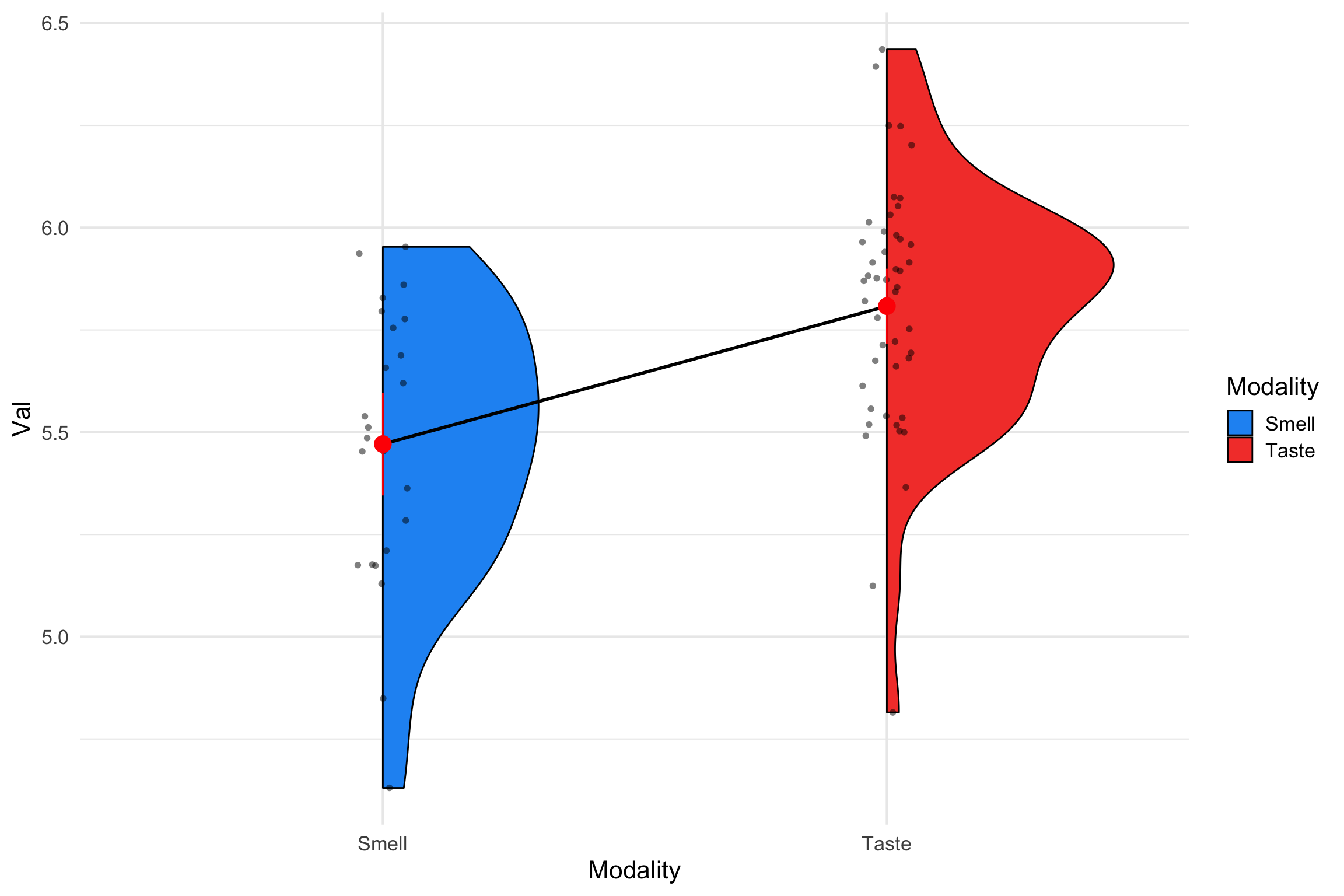
There was a statistically significant difference between Smell (M =5.47) and Taste Words (M = 5.81) in valence ratings , b = -.33, t =-4.33, 95% CI [-0.49, -0.13], p <.001 . Taste words were rated as more pleasant than smell words.

t-test

Same results!

t.test(Val ~ Modality, data=senses_filt, var.equal=TRUE) %>% tidy() %>%
  kable()

estimate	estimate1	estimate2	statistic	p.value	parameter	conf.low	conf.high	method	alternative
-0.3371123	5.471012	5.808124	-4.325684	4.95e-05	70	-0.4925442	-0.1816804	Two Sample t-test	two.sided

Multiple Levels

Linear models with multiple levels

So far we have only been looking at two levels
We easily can extend linear modeling approach to multiple levels
Let’s go back to our sense data
- Before filtering it down to 2 senses it had 5 senses!

glimpse(senses)

Rows: 405
Columns: 3
$ Word     <chr> "abrasive", "absorbent", "aching", "acidic", "acrid", "adhesi…
$ Modality <chr> "Touch", "Sight", "Touch", "Taste", "Smell", "Touch", "Taste"…
$ Val      <dbl> 5.398113, 5.876667, 5.233370, 5.539592, 5.173947, 5.240000, 5…

Treatment/dummy coding: multilevel factors

lm_all <- lm(Val~Modality, data=senses)

term	estimate	std.error	statistic	p.value
(Intercept)	5.5796631	0.0188944	295.307709	0.0000000
ModalitySmell	-0.1086515	0.0564307	-1.925396	0.0548885
ModalitySound	-0.1744704	0.0375767	-4.643046	0.0000047
ModalityTaste	0.2284608	0.0431387	5.295957	0.0000002
ModalityTouch	-0.0452281	0.0373697	-1.210289	0.2268828

What is going on here? There are only 4 levels, but we actually have 5 levels.

Dummy Coding Extension

Create one fewer dummy codes than levels (K (number of levels)-1)
Choose one of your levels as baseline and assign all zeros for this level across each dummy code
For first dummy code, assign 1 to first group and 0s for rest of levels

For the second dummy code, assign 1 to second group and 0s for rest of levels
For third dummy code, assign 1 to third group and 0s for rest of levels
For fourth dummy code, assign 1 to fourth group and 0s for rest of levels

Dummy Coding Extension

	.Smell-Sight	.Sound-Sight	.Taste-Sight	.Touch-Sight
Sight	0	0	0	0
Smell	1	0	0	0
Sound	0	1	0	0
Taste	0	0	1	0
Touch	0	0	0	1

Dummy Coding Extension

\[ \begin{align*} \operatorname{Val} &= b + b_{1}(\operatorname{Modality}_{\operatorname{Smell}}) \\ &\quad + b_{2}(\operatorname{Modality}_{\operatorname{Sound}}) \\ &\quad + b_{3}(\operatorname{Modality}_{\operatorname{Taste}}) \\ &\quad + b_{4}(\operatorname{Modality}_{\operatorname{Touch}}) + e \end{align*} \]

Dummy Coding Extension

senses_treatment  <- senses %>%
  mutate(mod_treat = faux::contr_code_treatment(Modality))
         
senses_treatment_lm <- lm(Val~mod_treat,  data=senses_treatment)

term	estimate	std.error	statistic	p.value
(Intercept)	5.5796631	0.0188944	295.307709	0.0000000
mod_treat.Smell-Sight	-0.1086515	0.0564307	-1.925396	0.0548885
mod_treat.Sound-Sight	-0.1744704	0.0375767	-4.643046	0.0000047
mod_treat.Taste-Sight	0.2284608	0.0431387	5.295957	0.0000002
mod_treat.Touch-Sight	-0.0452281	0.0373697	-1.210289	0.2268828

Sum Coding

Intercept = grand mean
Estimates = level vs. grand mean
- Assign 1 to target level, -1 to non-target level, 0 dropped

Sum Coding

	.Sight-intercept	.Smell-intercept	.Sound-intercept	.Taste-intercept
Sight	1	0	0	0
Smell	0	1	0	0
Sound	0	0	1	0
Taste	0	0	0	1
Touch	-1	-1	-1	-1

Sum Coding

senses_sum <- senses %>%
  mutate(sum = contr_code_sum(Modality)) 

lm_sum_coding <- lm(Val~sum, data=senses_sum)

term	estimate	std.error	statistic	p.value
(Intercept)	5.5596852	0.0164717	337.5305008	0.0000000
sum.Sight-intercept	0.0199778	0.0220344	0.9066657	0.3651295
sum.Smell-intercept	-0.0886737	0.0443596	-1.9989743	0.0462873
sum.Sound-intercept	-0.1544925	0.0300719	-5.1374316	0.0000004
sum.Taste-intercept	0.2484387	0.0342591	7.2517565	0.0000000

Deviation coding

Intercept = grand mean
Estimates = deviation/difference between level and reference level
- The target level gets:

\[ \frac{k-1}{k} \]

Any non-target level gets:

\[ -\frac{1}{k} \]

Deviation coding

## deviation coding
## baseline Sight it comes first in alphabet
dat_dev <- senses %>%
  mutate(SmellvSight = if_else(Modality == "Smell", 4/5, -1/5), # target A2
         SoundvSight = if_else(Modality == "Sound", 4/5, -1/5), 
         TastevSight = if_else(Modality=="Taste", 4/5, -1/5), 
         TouchvSight = if_else(Modality=="Touch", 4/5, -1/5))
         # target A3
# fit lm with new codes

Deviation coding

	.Smell-Sight	.Sound-Sight	.Taste-Sight	.Touch-Sight
Sight	-0.2	-0.2	-0.2	-0.2
Smell	0.8	-0.2	-0.2	-0.2
Sound	-0.2	0.8	-0.2	-0.2
Taste	-0.2	-0.2	0.8	-0.2
Touch	-0.2	-0.2	-0.2	0.8

Deviation coding

senses_dev <- senses  %>% 
  mutate(new=contr_code_anova(Modality))

dev_lm <- lm(Val~new, data=senses_dev)

term	estimate	std.error	statistic	p.value
(Intercept)	5.5596852	0.0164717	337.530501	0.0000000
new.Smell-Sight	-0.1086515	0.0564307	-1.925396	0.0548885
new.Sound-Sight	-0.1744704	0.0375767	-4.643046	0.0000047
new.Taste-Sight	0.2284608	0.0431387	5.295957	0.0000002
new.Touch-Sight	-0.0452281	0.0373697	-1.210289	0.2268828

DIY Contrasts

Rule 1: Groups coded with positive weights compared to groups with negative wights
Rule 2: The sum of weights you use should be zero
Rule 3: if a group is not involved in a comparison, assign it a weight of 0
Rule 4: Initial weight assigned to groups should be equal to # groups in opposite chunk of variation
Rule 5: To get final weights, divide initial weight by number of groups with non-zero weights.

Planned Contrast Example

Chemical vs. Non-chemical senses

Smell and Taste Sight, Touch, Sound Contrast

Positive Negative Sign of weight

3 2 Magnitude

3,3 2, 2, 2 Initial weight

3/5, 3/5 -2/5, -2/5, -2/5 Final weight

Smell and Taste	Sight, Touch, Sound	Contrast
Positive	Negative	Sign of weight
3	2	Magnitude
3,3	2, 2, 2	Initial weight
3/5, 3/5	-2/5, -2/5, -2/5	Final weight

Planned Contrast Example

TasteSmellVsOthers = c(-2/5, 3/5, -2/5, 3/5, -2/5)  # Comparing taste and smell to sight, touch, sound

mat=cbind(TasteSmellVsOthers)

#bind contrasts
#assign contrasts to factor
senses$Modality <- as.factor(senses$Modality)

#assign contrast weights
contrasts(senses$Modality)<-mat
#run model

The General Linear F-Test

3 or more groups
- Analysis of Variance (ANOVA)
We can think about the hypotheses for the overall test being:

\[H_0: \mu_1 = \mu_2 = \mu_3 = \mu_4 = \mu_5\]\[H_1: b_1 \neq b_2 \neq b_3 \neq b_4 \neq b_5\]\[H_1: \mu_1 \neq \mu_2 \neq \mu_3 \neq \mu_4 \neq \mu_5\]

Hello Again Sums of Squares

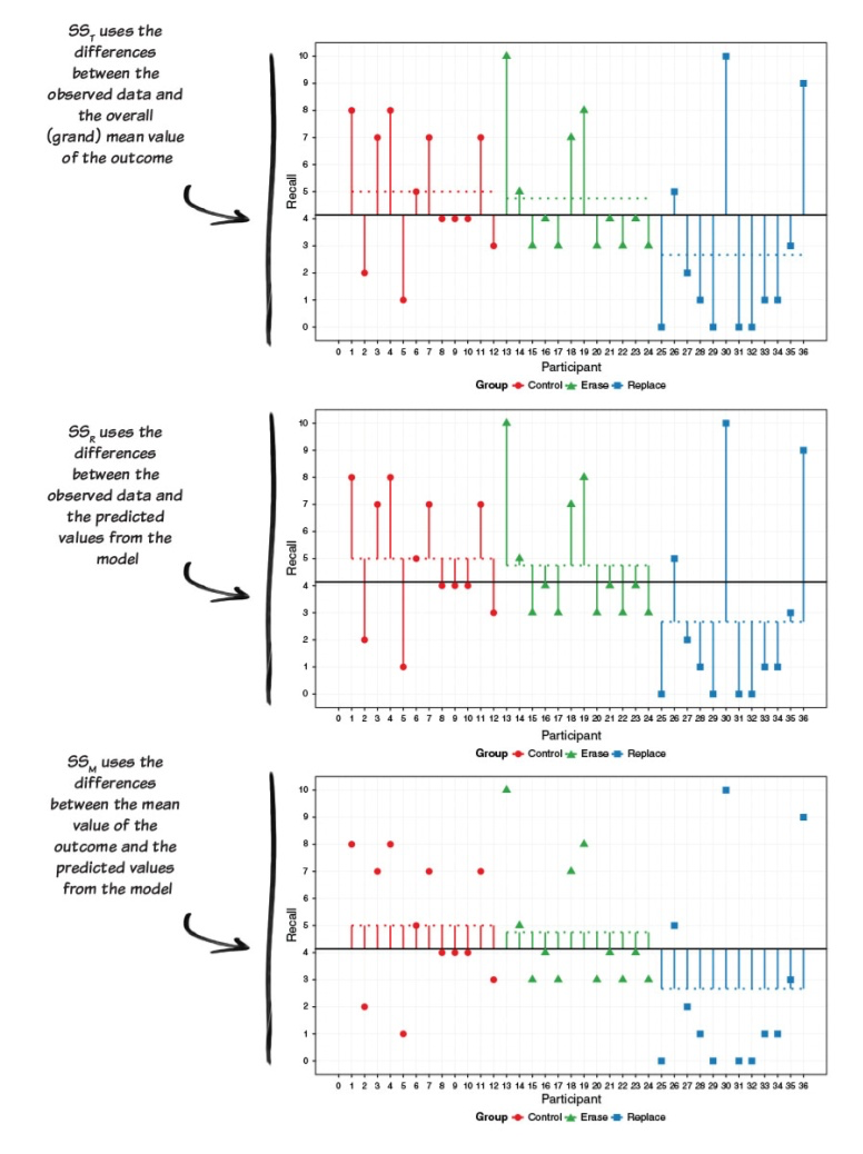
Field “Adventures in Statistics”

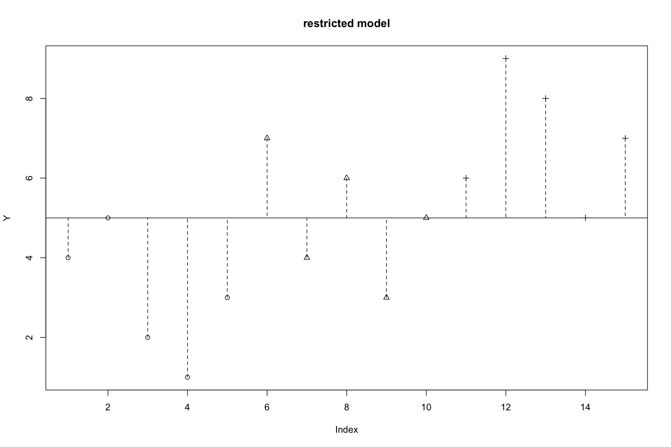
Empty Model

\[Y_{ij} = \mu + \epsilon\]

Restricted model (empty model): each score \(Y_{ij}\)is the result of a single population mean plus random error

\[SS_{error}(empty)=\sum(y_i-\bar{y})^2=SS_{total}\]

where:

\(y_i\) = observed value \(\bar{y}\) = mean value

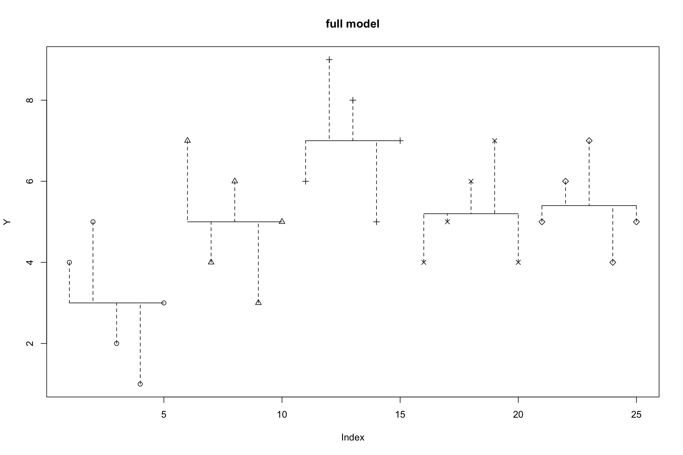
Full Model

\(Y_{ij} = \mu_j + e_{ij}\)

Full model (all predictors/levels): each score \(Y_{ij}\) is the result of a different group mean plus random error

\(SS_{error}(Full)=\sum(y_{ij}-\hat{y}_{ij})^2 = \\ SS_{unexplained}\)

where:

\(i\) = Person \(j\) = Group \(y_i\) = Observed value \(\hat{y}\) = Value estimated by regression line

F-ratio

F-ratio is measure of signal to noise

\[\begin{aligned} &&df_{empty} = N - 1\\ &&df_{full} = N - p\\ &&SSE_{empty}=SS_{total}\\&&SSE_{full}=SS_{unexplained}\end{aligned}\]

F-ratio

\[F = \frac{SS_{total}-SS_{unexplained}/{df_{empty}-df_{full}} (p-1)}{SS_{unexplained}/df_{full}(N-p)} = \frac{MS_{explained}}{MS_{unexplained}}\]

ANOVA Table

aov1<-aov(Val~ NULL, data=senses)
aov2 <- aov(Val~Modality, data=senses)
#anova(aov1, aov2) compare two models 
aov_em <- aov(Val~Modality, data=senses)

parameters::model_parameters(aov_em) %>%
  kable()

Parameter	Sum_Squares	df	Mean_Square	F	p
Modality	4.814548	4	1.2036370	17.02801	0
Residuals	28.274280	400	0.0706857	NA	NA

The Modality factor is significant. Now what?

Post-Hoc Comparisons

The second best package ever created: emmeans
Allows one to extract means for the model and also test comparisons of interest

Pairwise tests

Get means

# get pairwise tests between all groups
#specs = factor
emmeans::emmeans(aov_em, specs = "Modality")%>%
  kable()%>%
  kable_styling(font_size = 24) %>%
 column_spec(2, color = "white",
              background = "red")

Modality	emmean	SE	df	lower.CL	upper.CL
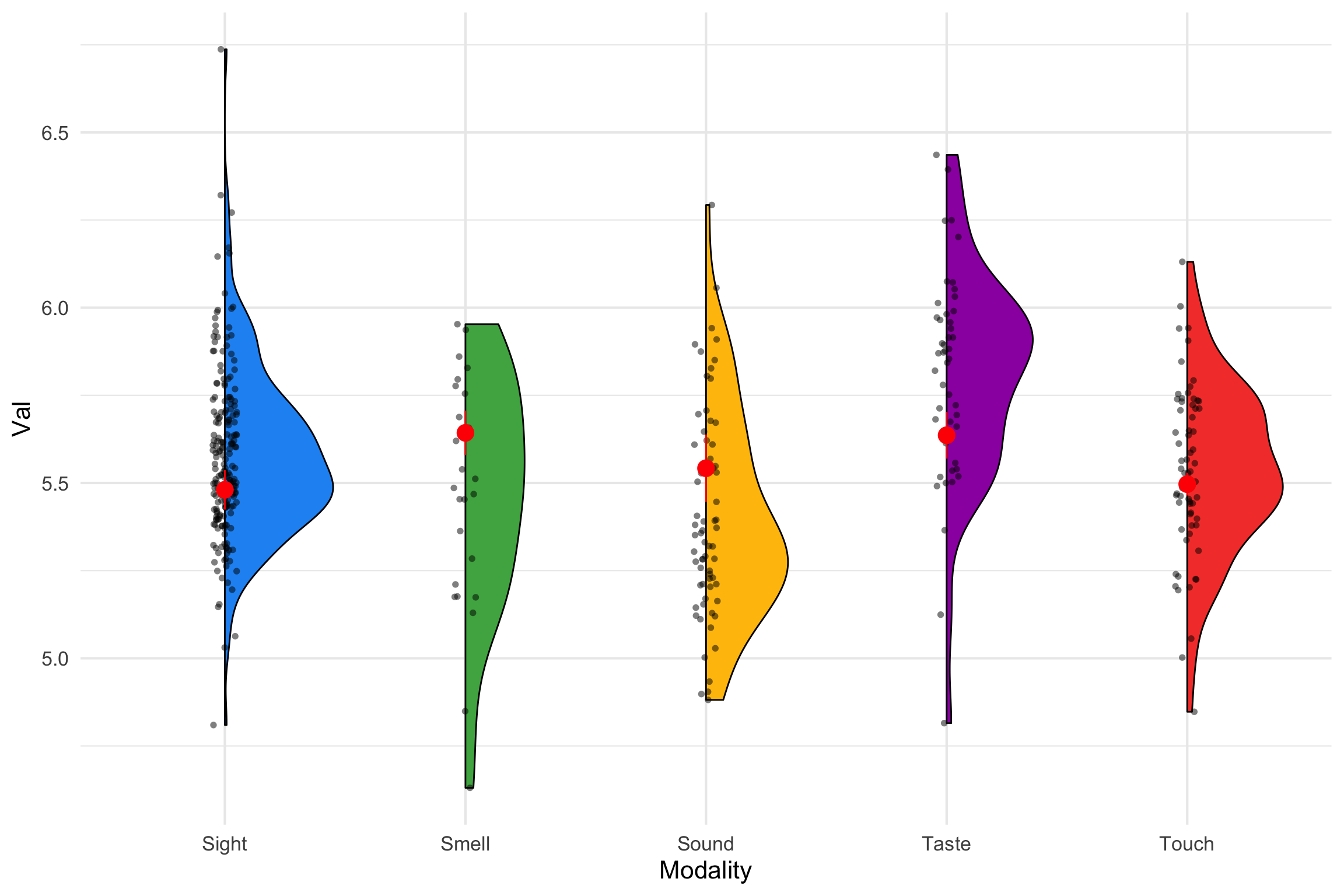
Sight	5.480531	0.0286568	400	5.424194	5.536867
Smell	5.643016	0.0323027	400	5.579511	5.706520
Sound	5.542073	0.0489734	400	5.445796	5.638351
Taste	5.636120	0.0339626	400	5.569352	5.702887
Touch	5.496687	0.0164950	400	5.464259	5.529115

Pairwise tests

and pairwise comparisons

# get pairwise tests between all groups
means1 = emmeans::emmeans(aov_em, specs = "Modality")

knitr::kable(pairs(means1)) %>%
  kable_styling(font_size = 24) %>%
 column_spec(2, color = "white",
              background = "red")

contrast	estimate	SE	df	t.ratio	p.value
Sight - Smell	-0.1624852	0.0405212	400	-4.0098820	0.0006890
Sight - Sound	-0.0615426	0.0705333	400	-0.8725316	0.9068515
Sight - Taste	-0.1555890	0.0370300	400	-4.2017062	0.0003145
Sight - Touch	-0.0161562	0.0185165	400	-0.8725316	0.9068515
Smell - Sound	0.1009426	0.0603593	400	1.6723634	0.4522890
Smell - Taste	0.0068962	0.0079036	400	0.8725316	0.9068515
Smell - Touch	0.1463290	0.0347012	400	4.2168260	0.0002952
Sound - Taste	-0.0940464	0.0669883	400	-1.4039239	0.6254936
Sound - Touch	0.0453864	0.0520169	400	0.8725316	0.9068515
Taste - Touch	0.1394328	0.0350160	400	3.9819749	0.0007701

Planned Comparisons

contr <- list(
    nonchem_vs_chem = c(-1/3, 1/2, -1/3, 1/2, -1/3))

emmeans::emmeans(aov_em, specs = "Modality") %>% contrast(method=contr) %>% 
  summary(infer=TRUE) %>%
  kable()

contrast	estimate	SE	df	lower.CL	upper.CL	t.ratio	p.value
nonchem_vs_chem	0.1331375	0.0368135	400	0.0607654	0.2055096	3.61654	0.0003368

Multiple Comparisons

We want our tests to find true positives and true negatives
Multiple comparisons
- Family-wise error rate

\[ FWER = 1 - (1 - \alpha)^k \]

k = number of comparisons

\(\alpha\)-inflation
- Testing each new pairwise comparison is costly

Bonferroni

\[\alpha / m\]

Where:
- m = number f comparisons
- \(\alpha\) = Level of significance
Controls for false positives (Type I errors)
Overly conservative
- Leads to false negatives (Type II errors)

Report adjusted p-values
- Multiple each by # tests

pvals = c(0.01,0.02,0.04)
p.adjust(pvals,method ="bonferroni", n = length(pvals))

[1] 0.03 0.06 0.12

Holm-Bonferroni

Strikes a balance between Type I and Type II errors

Sort p-values from smallest to largest

pvals = c(0.01,0.02,0.04)

Test whether p < \(\frac {\alpha} {m+ 1-k}\)

If so, reject and move to the next

Typically you report the adjusted p-value
- Just multiply your p-value by the adjusted alpha’s denominator

pvals = c(0.01,0.02,0.04)
p.adjust(pvals,method ="holm",n = length(pvals))

[1] 0.03 0.04 0.04

Many Multiple Comparison Corrections

Tukey
Scheffe
Dunnett
Fisher’s LSD (least significant difference)
Newman-Keuls

Note

Find what your field does and, more importantly, justify your decisions

`emmeans`

Correct p-values for multiple comparisons using the adjust argument

# get means
em_aov <- emmeans(aov_em, specs = "Modality")
# get pairwise comparisons
em_aov_pairs <- pairs(em_aov, adjust = "bonf")

contrast	estimate	SE	df	t.ratio	p.value
Sight - Smell	-0.1624852	0.0405212	400	-4.0098820	0.0007249
Sight - Sound	-0.0615426	0.0705333	400	-0.8725316	1.0000000
Sight - Taste	-0.1555890	0.0370300	400	-4.2017062	0.0003270
Sight - Touch	-0.0161562	0.0185165	400	-0.8725316	1.0000000
Smell - Sound	0.1009426	0.0603593	400	1.6723634	0.9523463
Smell - Taste	0.0068962	0.0079036	400	0.8725316	1.0000000
Smell - Touch	0.1463290	0.0347012	400	4.2168260	0.0003067
Sound - Taste	-0.0940464	0.0669883	400	-1.4039239	1.0000000
Sound - Touch	0.0453864	0.0520169	400	0.8725316	1.0000000
Taste - Touch	0.1394328	0.0350160	400	3.9819749	0.0008118

`emmeans`

Adjust CIs for multiple comparisons

emmeans1 <- emmeans::emmeans(aov_em, specs = "Modality")

emmeans1_pair <- pairs(emmeans1, adjust ="holm") %>% 
#get confidence intervals
confint(emmeans1_pair, adjust="bonf")

contrast	estimate	SE	df	lower.CL	upper.CL
Sight - Smell	-0.1624852	0.0405212	400	-0.2768640	-0.0481063
Sight - Sound	-0.0615426	0.0705333	400	-0.2606364	0.1375513
Sight - Taste	-0.1555890	0.0370300	400	-0.2601132	-0.0510648
Sight - Touch	-0.0161562	0.0185165	400	-0.0684224	0.0361101
Smell - Sound	0.1009426	0.0603593	400	-0.0694330	0.2713182
Smell - Taste	0.0068962	0.0079036	400	-0.0154133	0.0292057
Smell - Touch	0.1463290	0.0347012	400	0.0483781	0.2442798
Sound - Taste	-0.0940464	0.0669883	400	-0.2831338	0.0950409
Sound - Touch	0.0453864	0.0520169	400	-0.1014413	0.1922140
Taste - Touch	0.1394328	0.0350160	400	0.0405934	0.2382722

ANOVA Write-up

Factor
- Significance tests (F, degrees of freedom, p, effect size)
Post-hoc comparisons
- Difference
- Significance tests (t, degrees of freedom, p, effect size)
- \(\alpha\)-adjustment used
- Adjusted p-value

Plotting Group Means

Wrap-up

Linear models can be easily extended to categorical predictors
- Interpretation of intercept and slope are a bit different
  - Depends on coding scheme you use
- Interpretation of test statistics and statistical significance are the same
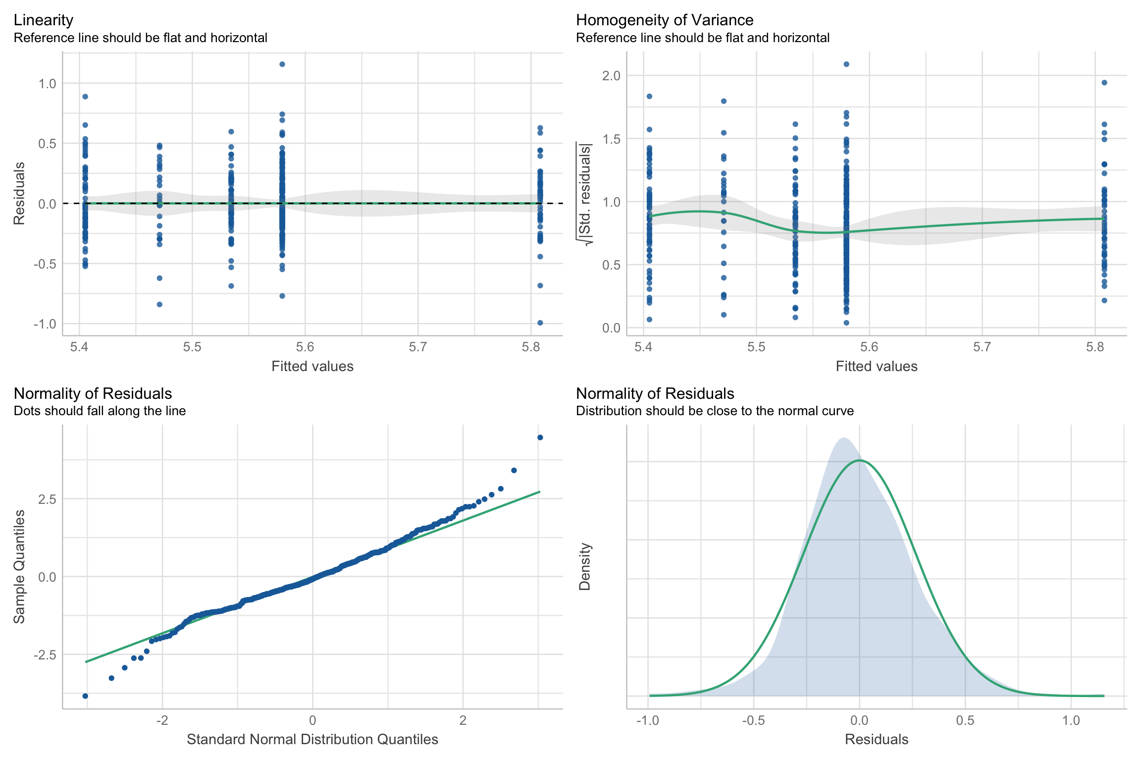
  - So are assumptions checks!

Assumption checks

mod_check <- lm(Val~Modality, data=senses)

performance::check_model(mod_check, check=c("normality", "linearity", "homogeneity", "qq"))

Next Week

Effect size and power analysis!