Crash Course in R

Princeton University

Jason Geller, PH.D.

2023-09-10

Packages

Package
base
gt
here
janitor
knitr
palmerpenguins
rmarkdown
skimr
tidyverse

Objective

Get you familiar with R
- Understand basic terminology and concepts
- Learn how to run commands
- Manipulate data
- Load and save data/scripts/QMD/RMD

It’s scary

Note

You can learn R!
You will get frustrated
You will get errors that don’t help or make sense
- Google is your friend
  - Try googling the specific error message first
  - Then try googling your specific function and the error
  - Try a bunch of different search terms.
- ChatGPT (use wisely)
- Me :)

Outline

Why R
IDE
R commands, data structures, and functions
Tidyverse & the pipe operator
Reading in data
Manipulating data
Saving data

Why R?

Free and open-source
Flexibility
Programming language (not point-and-click)
Excellent graphics (via ggplot2)

Easy to generate reproducible reports (markdown and quarto)
Easy to integrate with other tools and programs
Inclusive community
Marketability

Outline

Why R?
IDE
R commands, data structures, and functions
Tidyverse & the pipe operator
Multiple functions
Reading in data
Saving R scripts

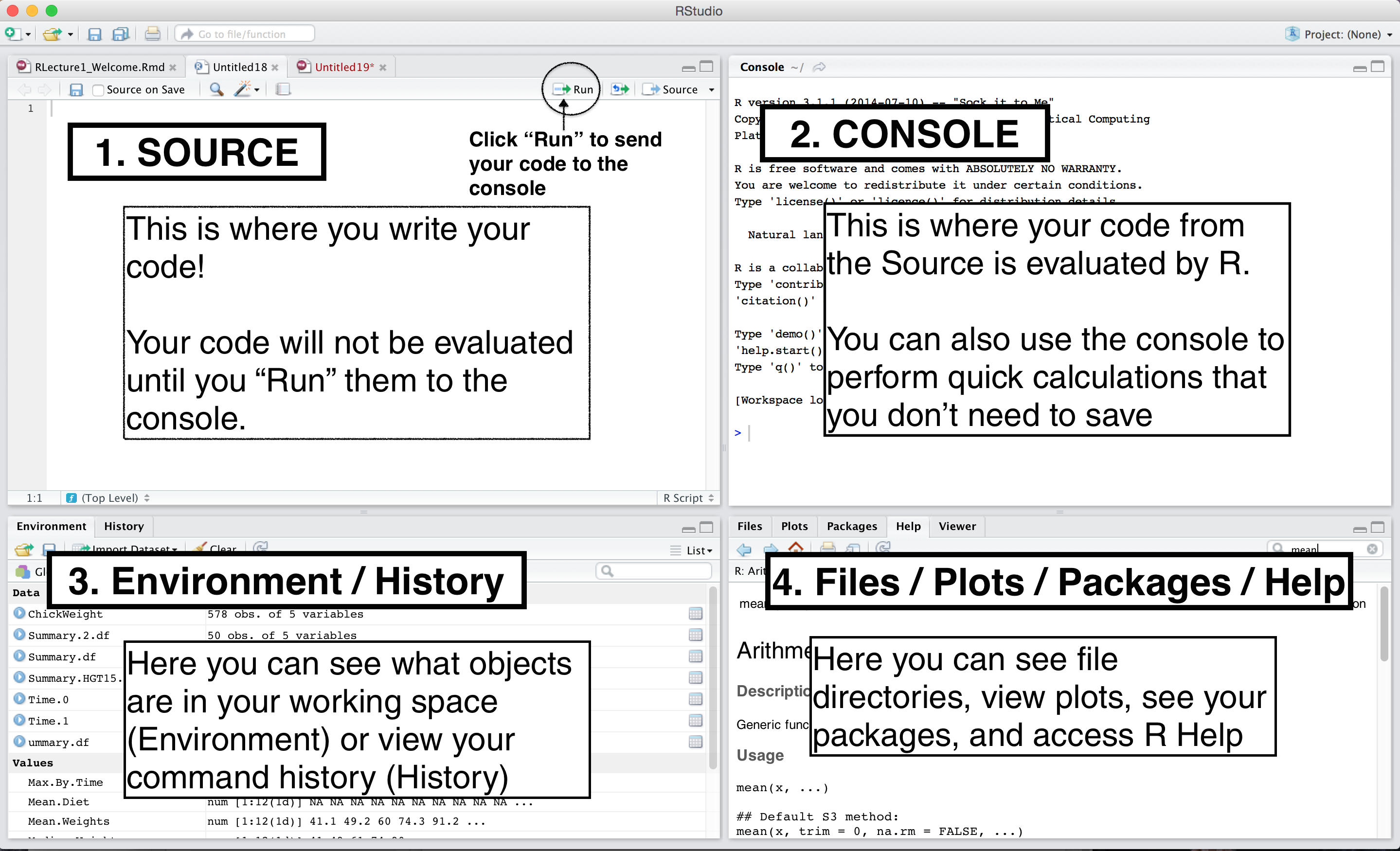
RStudio IDE

Make it your own!

Outline

Why R?
RStudio
R commands, data structures, and functions
Tidyverse & the pipe operator
Reading in data
Saving R scripts

Commands

Commands are the code that you tell R to do for you
They can be very simple or complex
Computers do what you tell them to do. Mistakes happen!
- Maybe it’s a typo, maybe it’s a misunderstanding of what the code does
You can type a command directly into the console
You can type in a document (Script or Markdown/Quarto) and tell it to then run in the console

X <- 4

Commands

> indicates the console is ready for more code
+ indicates that you haven’t finished a code block
Capitalization and symbols matter
Hit the up arrow – you can scroll through the last commands that were run
Hit the tab key – you’ll get a list of variable names and options to select from
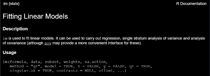
Use the ? followed by a command to learn more about it

Comments

You can make comments on your code using the # symbol
Comments are not processed by R, they provide documentation of your code for humans
Feel free to comment your personal code as much as you need to in order to understand it
Try to make your code clear enough that it can be understood even without comments

#this does something
#this does not work because I am stupid
x=4 #assign 4 to x

Assignment

Few different way to assign values to objects

#left arrow operator
x <- 4

The arrow <- is called an ASSIGNMENT OPERATOR, and tells R to save an object called x that has the value of 4
- Even -> (please don’t do this)
Can use = if you want

Objects and values

We will use the terms object and variable a lot when talking about code in this class
Objects are things you save in your environment (like a set of numbers, a dataset, or a regression model)
Variable refers to columns of a data frame and to data variables that we use in models

Vectors

Think of it as a row or column in a spreadsheet
Allows same classes to be concatenated together
- Numeric

x <-  c(2,6,16)

x

[1]  2  6 16

Vectors

Character

x <- c("cat", "bat")

gender <- c("male", "female")

Factors

gender <- as.factor(gender)

gender

[1] male   female
Levels: female male

Logical

x==7

[1] FALSE FALSE

Data frames

A data frame is like an Excel spreadsheet. It is two-dimensional with rows and columns.

Instead of creating a number of vectors we store all the vectors into a single DF
Can store numeric data (phone number, postal code, coordinates, etc.), float data (internet IP address, etc.), logical data (wants to receive ads: FALSE/TRUE, etc.), etc

car_model <- c("Ford Fusion", "Hyundai Accent", "Toyota Corolla")
car_price <- c(25000, 16000, 18000)
car_mileage <- c(27, 36, 32)

cars_df <- data.frame(model=car_model, price=car_price, mileage=car_mileage)

cars_df %>%
  knitr::kable()

model	price	mileage
Ford Fusion	25000	27
Hyundai Accent	16000	36
Toyota Corolla	18000	32

Tibbles

Modern take on data frames
- Tidy data!
  - Each variable forms a column
  - Each observation forms a row
  - Each cell is a single measurement
Only prints few rows
Never changes your input’s type or name

Matrices

Matrices are vectors with dimensions (like a 2X5)
All the data must be the same type

myMatrix <- matrix(data = 1:10,
                   nrow = 5,
                   ncol = 2)
myMatrix

     [,1] [,2]
[1,]    1    6
[2,]    2    7
[3,]    3    8
[4,]    4    9
[5,]    5   10

Lists

While vectors are one row of data, we might want to have multiple rows or types
With a vector, it is key to understand they have to be all the same type
Lists are a grouping of variables that can be multiple types (between list items) and can be different lengths
Often function output is saved as a list for this reason
They usually have names to help you print out just a small part of the list

library(palmerpenguins)

output <- lm(flipper_length_mm ~ bill_length_mm, data = penguins)
str(output)

List of 13
 $ coefficients : Named num [1:2] 126.68 1.69
  ..- attr(*, "names")= chr [1:2] "(Intercept)" "bill_length_mm"
 $ residuals    : Named num [1:342] -11.766 -7.442 0.206 4.29 -3.104 ...
  ..- attr(*, "names")= chr [1:342] "1" "2" "3" "5" ...
 $ effects      : Named num [1:342] -3715.57 170.39 1.03 5.35 -2.22 ...
  ..- attr(*, "names")= chr [1:342] "(Intercept)" "bill_length_mm" "" "" ...
 $ rank         : int 2
 $ fitted.values: Named num [1:342] 193 193 195 189 193 ...
  ..- attr(*, "names")= chr [1:342] "1" "2" "3" "5" ...
 $ assign       : int [1:2] 0 1
 $ qr           :List of 5
  ..$ qr   : num [1:342, 1:2] -18.4932 0.0541 0.0541 0.0541 0.0541 ...
  .. ..- attr(*, "dimnames")=List of 2
  .. .. ..$ : chr [1:342] "1" "2" "3" "5" ...
  .. .. ..$ : chr [1:2] "(Intercept)" "bill_length_mm"
  .. ..- attr(*, "assign")= int [1:2] 0 1
  ..$ qraux: num [1:2] 1.05 1.04
  ..$ pivot: int [1:2] 1 2
  ..$ tol  : num 1e-07
  ..$ rank : int 2
  ..- attr(*, "class")= chr "qr"
 $ df.residual  : int 340
 $ na.action    : 'omit' Named int [1:2] 4 272
  ..- attr(*, "names")= chr [1:2] "4" "272"
 $ xlevels      : Named list()
 $ call         : language lm(formula = flipper_length_mm ~ bill_length_mm, data = penguins)
 $ terms        :Classes 'terms', 'formula'  language flipper_length_mm ~ bill_length_mm
  .. ..- attr(*, "variables")= language list(flipper_length_mm, bill_length_mm)
  .. ..- attr(*, "factors")= int [1:2, 1] 0 1
  .. .. ..- attr(*, "dimnames")=List of 2
  .. .. .. ..$ : chr [1:2] "flipper_length_mm" "bill_length_mm"
  .. .. .. ..$ : chr "bill_length_mm"
  .. ..- attr(*, "term.labels")= chr "bill_length_mm"
  .. ..- attr(*, "order")= int 1
  .. ..- attr(*, "intercept")= int 1
  .. ..- attr(*, "response")= int 1
  .. ..- attr(*, ".Environment")=<environment: R_GlobalEnv> 
  .. ..- attr(*, "predvars")= language list(flipper_length_mm, bill_length_mm)
  .. ..- attr(*, "dataClasses")= Named chr [1:2] "numeric" "numeric"
  .. .. ..- attr(*, "names")= chr [1:2] "flipper_length_mm" "bill_length_mm"
 $ model        :'data.frame':  342 obs. of  2 variables:
  ..$ flipper_length_mm: int [1:342] 181 186 195 193 190 181 195 193 190 186 ...
  ..$ bill_length_mm   : num [1:342] 39.1 39.5 40.3 36.7 39.3 38.9 39.2 34.1 42 37.8 ...
  ..- attr(*, "terms")=Classes 'terms', 'formula'  language flipper_length_mm ~ bill_length_mm
  .. .. ..- attr(*, "variables")= language list(flipper_length_mm, bill_length_mm)
  .. .. ..- attr(*, "factors")= int [1:2, 1] 0 1
  .. .. .. ..- attr(*, "dimnames")=List of 2
  .. .. .. .. ..$ : chr [1:2] "flipper_length_mm" "bill_length_mm"
  .. .. .. .. ..$ : chr "bill_length_mm"
  .. .. ..- attr(*, "term.labels")= chr "bill_length_mm"
  .. .. ..- attr(*, "order")= int 1
  .. .. ..- attr(*, "intercept")= int 1
  .. .. ..- attr(*, "response")= int 1
  .. .. ..- attr(*, ".Environment")=<environment: R_GlobalEnv> 
  .. .. ..- attr(*, "predvars")= language list(flipper_length_mm, bill_length_mm)
  .. .. ..- attr(*, "dataClasses")= Named chr [1:2] "numeric" "numeric"
  .. .. .. ..- attr(*, "names")= chr [1:2] "flipper_length_mm" "bill_length_mm"
  ..- attr(*, "na.action")= 'omit' Named int [1:2] 4 272
  .. ..- attr(*, "names")= chr [1:2] "4" "272"
 - attr(*, "class")= chr "lm"

Indexing

Vectors can be indexed
- 1 not 0 (👀 Python)

x=c(1,2,3,4)
x[1] # ret first

[1] 1

x[-2] # everything but that number

[1] 1 3 4

x[1] <- 7 # Change values in vector
x

[1] 7 2 3 4

R as a calculator

Typing in a simple calculation show us the result

#add
608+ 28

[1] 636

#subtract
11527-283

[1] 11244

# divison
400/65

[1] 6.153846

#multiplication
2*4

[1] 8

#exponentiation
5^2

[1] 25

Functions

Take arguments, do something to them, and return the result
More complex calculations can be done with functions:
- What is square root of 64?

# sqrt function
# in parenthesis: what we want to perform function on
sqrt(64)

[1] 8

sr=function(a, b){
  c=a + b
  return(c)
}

sr(2,3)

Arguments

Some functions have settings (“arguments”) that we can adjust:
round(3.14)
- Rounds off to the nearest integer (zero decimal places)
round(3.14, digits=1)
- One decimal place

Getting Help

Help files

Exercise

Open a blank new script
To paste strings together you can use the paste() function (e.g., paste(“Hello”, “World”)). Use ?paste or Google “paste function in R” to get an idea of how to use this function.

2.1 Create three vectors. One vector should have three first names. The second vector should have 3 last names. Finally, the third vector should have 3 ages. Use the paste function to string together these vectors separated by a _
Modify the function below and instead of returning the sum, return the mean
```
mean=function(a, b){
  c=a + b
  return(c)
}
```

Outline

Why R
IDE
R commands & functions
Tidyverse & the pipe operator
Reading in data
Saving R scripts

Tidyverse and pipes

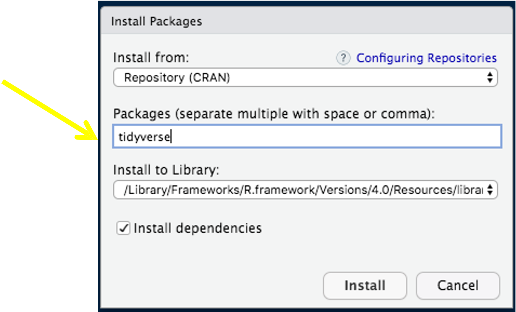
The tidyverse is an ecosystem of R packages designed for data science. All packages share an underlying design philosophy, grammar, and data structures.

Installing Tidyverse

install.packages(tidyverse)

Load package

library(tidyverse)

Pipes

tidyverse provides another interface to functions
- the pipe operator
  - Makes code easier to read and follow:
This:

a %>% 
  round()

Can be converted into:
- Start with a and then round
|> pipe is slowly becoming more popular

Multiple functions

Pipe operator makes it easy to do multiple functions in a row

-16 %>%
  abs()%>%
  sqrt()


-16 |> 
  abs() |>
  sqrt()

What is this doing?

Outline

Why R
IDE
R commands & functions
Tidyverse & the pipe operator
Reading in data
Saving R scripts

Reading in data

Download the file

General form: dataframe.name <-read_csv('filename')

Reading other file types

Excel

library(readxl)

fac<-  read_excel('/Users/jg/Desktop/experiment.xlsx', sheet=2)
# excel files can have multiple sheets

SPSS

library(haven)

fac<-  read_spss('/Users/jg/Desktop/experiment.spss')

Working directories

Here package
- Here helps set relative as opposed to absolute paths

Here

#setwd("your path here")

#install here
library(here)

# here

here::here()

[1] "/Users/jasongeller/Documents/GitHub/PSY503-F2023"

# can use with read.csv

Loading the data

Note

Always create an R project before you start

Aside: naming conventions

Variable names in DFs are case-sensitive
Variable names can contain letters, numbers, underscores “_” and periods “.”
- In most cases you should use snake_case to name objects
- use_an_underscore_between_words
- Avoid periods
Names should be short and descriptive, with descriptive being the most important feature

Janitor

Loading the data

You can download data directly from OSF or Github
- https://osf.io/cmtxa

The faculty dataset contains aggregated data per faculty:

faculty: Business, Economics, Political Science, Sociology
students: number of students
profs: number of profs
salary: amount of salary
costs: amount of costs dataset entails demographic and school-related information on imaginary students, such as

Load data from OSF

Looking at data

fac%>%
  summary()

   faculty             students         profs           salary     
 Length:4           Min.   :162.0   Min.   :63.00   Min.   :54246  
 Class :character   1st Qu.:209.2   1st Qu.:72.75   1st Qu.:56516  
 Mode  :character   Median :244.5   Median :76.50   Median :61849  
                    Mean   :247.5   Mean   :73.75   Mean   :65309  
                    3rd Qu.:282.8   3rd Qu.:77.50   3rd Qu.:70642  
                    Max.   :339.0   Max.   :79.00   Max.   :83292  
     costs      
 Min.   :24965  
 1st Qu.:28471  
 Median :31493  
 Mean   :30370  
 3rd Qu.:33391  
 Max.   :33527

Looking at data

library(skimr)
fac%>%
  skim() %>% 
 gt()

skim_type	skim_variable	complete_rate	character.min	character.max	character.empty	character.n_unique	character.whitespace	numeric.mean	numeric.sd	numeric.p0	numeric.p25	numeric.p50	numeric.p75	numeric.p100	numeric.hist
character	faculty	1	8	17	0	4	0	NA	NA	NA	NA	NA	NA	NA	NA
numeric	students	1	NA	NA	NA	NA	NA	247.50	74.074287	162	209.25	244.5	282.75	339	▇▇▇▁▇
numeric	profs	1	NA	NA	NA	NA	NA	73.75	7.274384	63	72.75	76.5	77.50	79	▂▁▁▁▇
numeric	salary	1	NA	NA	NA	NA	NA	65309.00	13058.854084	54246	56516.25	61849.0	70641.75	83292	▇▁▃▁▃
numeric	costs	1	NA	NA	NA	NA	NA	30369.50	4023.686080	24965	28471.25	31493.0	33391.25	33527	▃▁▃▁▇

Looking at data

fac # whole dataset

# A tibble: 4 × 5
  faculty           students profs salary costs
  <chr>                <dbl> <dbl>  <dbl> <dbl>
1 Business               339    76  57273 33346
2 Economics              225    79  83292 33527
3 Political Science      264    63  66425 24965
4 Sociology              162    77  54246 29640

head(fac)

# A tibble: 4 × 5
  faculty           students profs salary costs
  <chr>                <dbl> <dbl>  <dbl> <dbl>
1 Business               339    76  57273 33346
2 Economics              225    79  83292 33527
3 Political Science      264    63  66425 24965
4 Sociology              162    77  54246 29640

tail(fac)

# A tibble: 4 × 5
  faculty           students profs salary costs
  <chr>                <dbl> <dbl>  <dbl> <dbl>
1 Business               339    76  57273 33346
2 Economics              225    79  83292 33527
3 Political Science      264    63  66425 24965
4 Sociology              162    77  54246 29640

Looking at data

# look at specific variables
table(fac$students)


162 225 264 339 
  1   1   1   1

# let's try another package
library("janitor")
tabyl(fac$students)

 fac$students n percent
          162 1    0.25
          225 1    0.25
          264 1    0.25
          339 1    0.25

Outline

Why R
IDE
R commands, data structures, and functions
Tidyverse & the Pipe Operator
Reading in data
Manipulating data
Saving R scripts

Manipulating data

dplyr is organized around verbs that manipulate data frames
Isolating data:
- select
- filter
- mutate
- summarize

Select

Palmer penguins

df = palmerpenguins::penguins

df %>% 
  head() %>%
  knitr::kable()

species	island	bill_length_mm	bill_depth_mm	flipper_length_mm	body_mass_g	sex	year
Adelie	Torgersen	39.1	18.7	181	3750	male	2007
Adelie	Torgersen	39.5	17.4	186	3800	female	2007
Adelie	Torgersen	40.3	18.0	195	3250	female	2007
Adelie	Torgersen	NA	NA	NA	NA	NA	2007
Adelie	Torgersen	36.7	19.3	193	3450	female	2007
Adelie	Torgersen	39.3	20.6	190	3650	male	2007

Select columns

The select command from dplyr allows you to subset columns matching strings:

select(df, sex, year) %>%
  head() %>% 
  knitr::kable()

sex	year
male	2007
female	2007
female	2007
NA	2007
female	2007
male	2007

Select helpers

Select columns

If you wanted it to be a single vector (not a tibble), use pull:

pull(select(df, sex))

  [1] male   female female <NA>   female male   female male   <NA>   <NA>  
 [11] <NA>   <NA>   female male   male   female female male   female male  
 [21] female male   female male   male   female male   female female male  
 [31] female male   female male   female male   male   female female male  
 [41] female male   female male   female male   male   <NA>   female male  
 [51] female male   female male   female male   female male   female male  
 [61] female male   female male   female male   female male   female male  
 [71] female male   female male   female male   female male   female male  
 [81] female male   female male   female male   male   female male   female
 [91] female male   female male   female male   female male   female male  
[101] female male   female male   female male   female male   female male  
[111] female male   female male   female male   female male   female male  
[121] female male   female male   female male   female male   female male  
[131] female male   female male   female male   female male   female male  
[141] female male   female male   female male   male   female female male  
[151] female male   female male   female male   male   female female male  
[161] female male   female male   female male   female male   female male  
[171] female male   male   female female male   female male   <NA>   male  
[181] female male   male   female female male   female male   female male  
[191] female male   female male   female male   male   female female male  
[201] female male   female male   female male   female male   female male  
[211] female male   female male   female male   female male   <NA>   male  
[221] female male   female male   male   female female male   female male  
[231] female male   female male   female male   female male   female male  
[241] female male   female male   female male   female male   male   female
[251] female male   female male   female male   <NA>   male   female male  
[261] female male   female male   female male   female male   <NA>   male  
[271] female <NA>   female male   female male   female male   male   female
[281] male   female female male   female male   female male   female male  
[291] female male   male   female female male   female male   female male  
[301] female male   female male   female male   female male   female male  
[311] male   female female male   female male   male   female male   female
[321] female male   female male   male   female female male   female male  
[331] female male   female male   male   female male   female female male  
[341] female male   male   female
Levels: female male

Filter

df %>% 
filter(sex=="male") %>%
  head()

# A tibble: 6 × 8
  species island    bill_length_mm bill_depth_mm flipper_length_mm body_mass_g
  <fct>   <fct>              <dbl>         <dbl>             <int>       <int>
1 Adelie  Torgersen           39.1          18.7               181        3750
2 Adelie  Torgersen           39.3          20.6               190        3650
3 Adelie  Torgersen           39.2          19.6               195        4675
4 Adelie  Torgersen           38.6          21.2               191        3800
5 Adelie  Torgersen           34.6          21.1               198        4400
6 Adelie  Torgersen           42.5          20.7               197        4500
# ℹ 2 more variables: sex <fct>, year <int>

Note, no $ or subsetting is necessary

Filter

You can have multiple logical conditions using the following:

== : equals to
! : not/negation
> / <: greater than / less than
>= or <=: greater than or equal to / less than or equal to
& : AND
| : OR
is.na(x): is NA
!is.na(x): is not NA

Common mistakes

Using = instead of ==

filter(df, sex=1)

Forgetting quotes

filter(df, Name==John)

filter(df, Name=="John")

Exercise

Return a df that only has NA for sex

Mutate

df %>% 
  #combines what is in species and #what is island together with #underscore
  mutate(spec_island=paste(species,island, sep="_")) %>%
  head()

# A tibble: 6 × 9
  species island    bill_length_mm bill_depth_mm flipper_length_mm body_mass_g
  <fct>   <fct>              <dbl>         <dbl>             <int>       <int>
1 Adelie  Torgersen           39.1          18.7               181        3750
2 Adelie  Torgersen           39.5          17.4               186        3800
3 Adelie  Torgersen           40.3          18                 195        3250
4 Adelie  Torgersen           NA            NA                  NA          NA
5 Adelie  Torgersen           36.7          19.3               193        3450
6 Adelie  Torgersen           39.3          20.6               190        3650
# ℹ 3 more variables: sex <fct>, year <int>, spec_island <chr>

Creating conditional (if-else) variables

A general function for creating new variables based on existing variables is the ifelse() function, which returns a value with the same shape as test which is filled with elements selected from either yes or no depending on whether the element of test is TRUE or FALSE.

ifelse(test, yes, no)

# test: an object which can be coerced
#to logical mode.
# yes: return values for true elements of test.
# no: return values for false elements of test.

Adding columns

Mutate combined with ifelse(condition, TRUE, FALSE), it can give you:

df = mutate(df, 
            island_num = ifelse(
              island=="Biscoe",
              "first_island", ifelse(
              island== "Dream", "second_island", 
              "third_island")
            )
)
head(df$island_num)

[1] "third_island" "third_island" "third_island" "third_island" "third_island"
[6] "third_island"

Case_when

df = mutate(df, 
            island_num = case_when(
              island=="Biscoe" ~ "first_island",
              island=="Dream" ~ "second_island",
              TRUE ~ "third_island"
            ))
df %>%
  select(island_num) %>%
  head() %>%
  knitr::kable()

island_num
third_island
third_island
third_island
third_island
third_island
third_island

Exercise

See if you can use the logical operators to manipulate our penguins data using %>%

All of the penguin data from year 2007
All of the female penguins
Get flipper length > 150
Select only the flipper length and species columns

Summarize

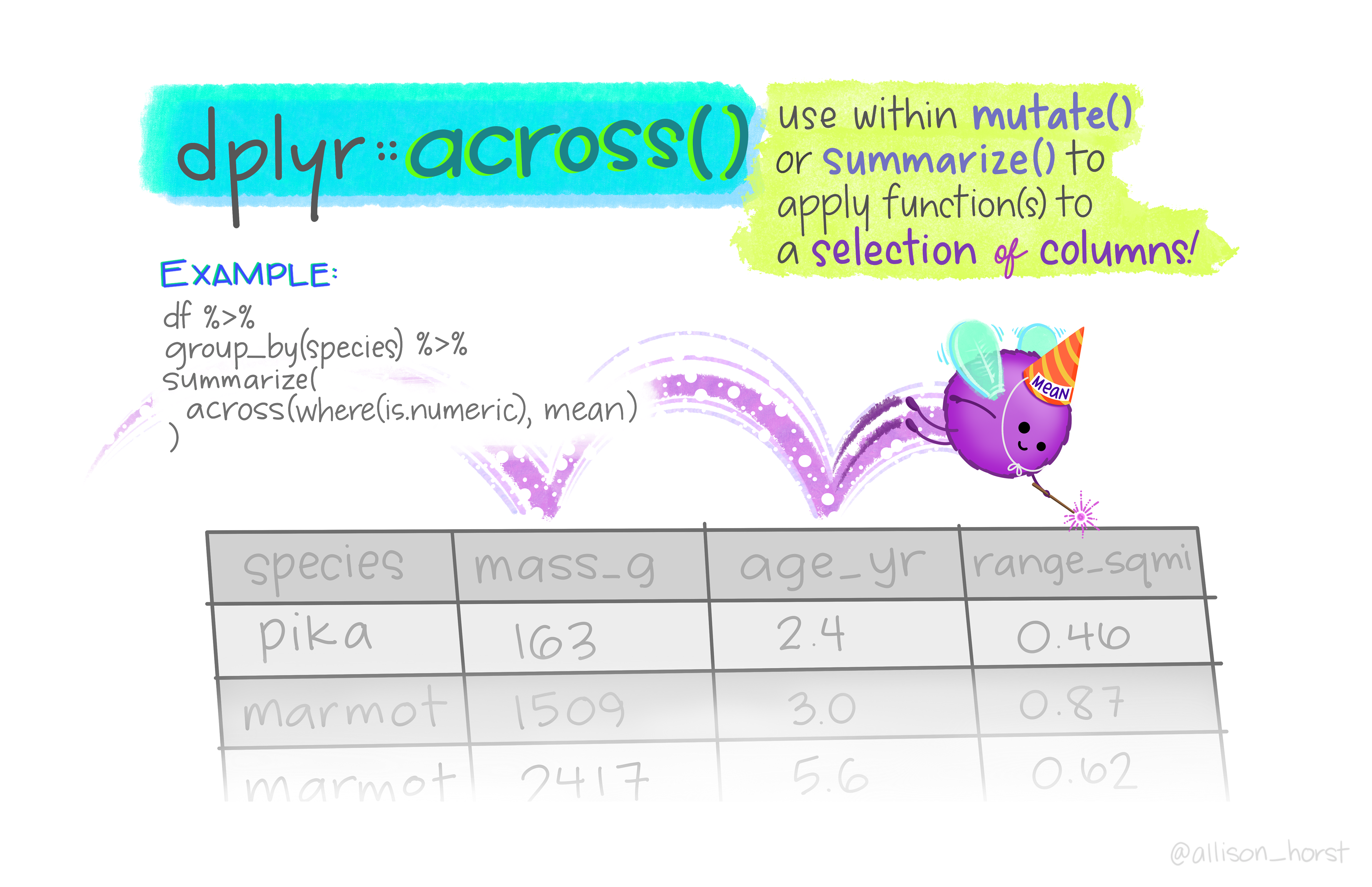
Create summary statistics (mean, median, SD, sum)
- Use with group_by

Outline

Why R
IDE
R commands & functions
Tidyverse & the pipe operator
Reading in data
Manipulating data
Saving R scripts

Saving files

write.csv(fac, file="df.csv")

write.table(fac, file="df.txt")

Wrapping up

You’ve learned:
- Some basic programming terminology
- Specific R defaults and issues
- Example functions and use cases
How do I get started?
- Practice!

Helpful websites

Google!
Cheat sheets (https://rstudio.cloud/learn/cheat-sheets)
Quick-R: www.statmethods.net
R documentation: www.rdocumentation.org
Swirl: www.swirlstats.com
Stack Overflow: www.stackoverflow.com
Learn Statistics with R: https://learningstatisticswithr.com/