Lab 10: Factorial Designs

Princeton University

Published

December 11, 2023

Research scenario

Based on subjects’ self-reports of rejection sensitivity (N = 80), a researcher divides subjects into two equal groups (low RS and high RS). Whereas half of the subjects in each group interact with a partner who displays a happy emotional expression during the interaction, the other half of the subjects in each group interact with a partner who displays a neutral emotional expression during the interaction. After the interaction, subjects are asked to rate the statement, “My interaction partner likes me”, on a scale from 1 (strongly disagree) to 7 (strongly agree).

Factor 1: Rejection Sensitivity

Low
High

Factor 2: Partner’s Emotional Expression

Neutral
Happy

Dependent Variable: Perceived Liking

Import & inspect the data

#load packages
library(tidyverse)
library(emmeans)
library(apaTables)
library(easystats)
library(broom)

Load the .csv file from the repository

reject <- read.csv("https://raw.githubusercontent.com/jgeller112/Lab10-Interactions-2/main/reject.csv")

Make sure the categorical variables are factors

str(reject)

'data.frame':   80 obs. of  4 variables:
 $ X      : int  1 2 3 4 5 6 7 8 9 10 ...
 $ rs     : chr  "Low " "Low " "Low " "Low " ...
 $ partner: chr  "Neutral " "Neutral " "Neutral " "Neutral " ...
 $ liking : int  4 4 4 5 5 5 5 5 5 5 ...

reject_cat <- reject  %>%
  mutate(rs_cat=as.factor(rs), partner_cat=as.factor(partner))

str(reject_cat)

'data.frame':   80 obs. of  6 variables:
 $ X          : int  1 2 3 4 5 6 7 8 9 10 ...
 $ rs         : chr  "Low " "Low " "Low " "Low " ...
 $ partner    : chr  "Neutral " "Neutral " "Neutral " "Neutral " ...
 $ liking     : int  4 4 4 5 5 5 5 5 5 5 ...
 $ rs_cat     : Factor w/ 2 levels "High ","Low ": 2 2 2 2 2 2 2 2 2 2 ...
 $ partner_cat: Factor w/ 2 levels "Happy ","Neutral ": 2 2 2 2 2 2 2 2 2 2 ...

Notice that by default R orders factor levels alphabetically. In our case, this means that High will be the reference group of rejection sensitivity and Happy will be the reference group of interaction partner’s emotional expression. However, it might be more intuitive to have Low and Neutral be the reference groups, respectively.

Reorder the levels

reject_cat <- reject_cat %>% 
  mutate(rs_cat = factor(rs, levels=c("Low ", "High ")),
         partner_cat = factor(partner,levels= c("Neutral ", "Happy ")))

Descriptive Statistics

How many Ps are there per condition?

reject_cat %>%
  group_by(rs_cat, partner_cat) %>%
  summarise(n=n())

# A tibble: 4 × 3
# Groups:   rs_cat [2]
  rs_cat  partner_cat     n
  <fct>   <fct>       <int>
1 "Low "  "Neutral "     20
2 "Low "  "Happy "       20
3 "High " "Neutral "     20
4 "High " "Happy "       20

Table of Means

The results of a factorial ANOVA are often represented in a table of means, which contains the means of each combination of conditions (the cell means) and means for the levels of each variable ignoring the other variables (the marginal means)

Table of Means

The apa.2way.table() function from the apaTables package is a very convenient way to get our cell means and marginal means. This function works for any type of 2-way ANOVA, regardless of the number of levels of your factors, e.g. it would work for a 3 x 3 ANOVA. All you need to do is indicate what the IV’s (aka factors) and DV are and specify show.marginal.means = TRUE.

Use apa.2way.table() to create a table for our data

apa.2way.table(iv1 = rs_cat, 
               iv2 = partner_cat, 
               dv = liking, 
               data = reject_cat,
               show.marginal.means = TRUE)



Table 0 

Descriptive Statistics For Liking In a 2(Rs_cat) X 2(Partner_cat) Design 

          partner_cat                               
             Neutral       Happy       Marginal     
   rs_cat           M   SD      M   SD        M   SD
     Low         5.55 1.05   6.00 0.73     5.78 0.92
    High         1.80 0.70   6.45 0.69     4.12 2.45
 Marginal        3.67 2.09   6.22 0.73              

Note. M = mean. SD = standard deviation. 
Marginal indicates the means and standard deviations pertaining to main effects.

Question: Which means are being compared in the main effect of rejection sensitivity?

4.12 and 5.78

Question: Which means are being compared in the main effect of interaction partner?

6.22 and 3.67

Question:Which means are involved in the interaction?

6.45, 6.00, 1.80, 5.55

Conduct the Factorial ANOVA

Using Regression: `lm`()

Run a dummy coded regression analysis

## your code here

model <- lm(liking ~ rs_cat * partner_cat, data = reject_cat) %>%
  tidy(conf.int = TRUE) 

model

# A tibble: 4 × 7
  term                  estimate std.error statistic  p.value conf.low conf.high
  <chr>                    <dbl>     <dbl>     <dbl>    <dbl>    <dbl>     <dbl>
1 "(Intercept)"            5.55      0.180     30.9  9.26e-45   5.19       5.91 
2 "rs_catHigh "           -3.75      0.254    -14.8  5.19e-24  -4.26      -3.24 
3 "partner_catHappy "      0.450     0.254      1.77 8.07e- 2  -0.0562     0.956
4 "rs_catHigh :partner…    4.20      0.359     11.7  1.21e-18   3.48       4.92

Interpret each of the regression coefficients

\(b_0\): The predicted Y value for the neutral, low group (M=5.55)
\(b_1\): The simple effect for the low vs. high group when neutral, b = -3.75, SE = 0.25, 95% CI[-4.26, -3.24], t = -14.75, p < .001.
\(b_2\): The simple effect for the neutral vs. happy group when low, b = 0.45, SE = 0.25, 95% CI[-4.26, -3.24], p > .05.
\(b_3\): The interaction between the rs and partner group, b = 4.20, SE = 0.36, 95% CI[-4.26, -3.24], p < .001.

Recoding

Obviously, the means being compared by b1 and b2 do not represent our main effects. The main effect of RS would be a comparison of the marginal means for the low and high conditions. The main effect of partner would be a comparison of the marginal means for the neutral and happy conditions.

With the way we have rs and partner coded in the model, the regression coefficient estimates don’t correspond simply to the mean difference between conditions. We can recode the factors so that the parameter estimates, b1 and b2, correspond to a test of the main effects.

Question: How should we code the levels of rejection sensitivity and partner emotion so that the parameter estimates, b1 and b2, correspond to a test of their main effects?

Devaition coding

Assign new codes to the levels of each factor

#change to dev coding
contrasts(reject_cat$rs_cat)<-c(0.5, -0.5)
contrasts(reject_cat$partner_cat)<-c(0.5, -0.5)

Re-run the analysis with newly coded factors

model_dev <- lm(liking ~ rs_cat * partner_cat, data = reject_cat) %>%
  tidy(conf.int = TRUE) 

model_dev

# A tibble: 4 × 7
  term                 estimate std.error statistic  p.value conf.low conf.high
  <chr>                   <dbl>     <dbl>     <dbl>    <dbl>    <dbl>     <dbl>
1 (Intercept)              4.95    0.0899     55.1  5.14e-63     4.77      5.13
2 rs_cat1                  1.65    0.180       9.18 6.03e-14     1.29      2.01
3 partner_cat1            -2.55    0.180     -14.2  4.64e-23    -2.91     -2.19
4 rs_cat1:partner_cat1     4.20    0.359      11.7  1.21e-18     3.48      4.92

Interpret the new model coefficients

\(b_0\): The grand mean across all cell means
\(b_1\): The main effect of rejection sensitivity, b = 1.65, SE = 0.18, 95% CI[-4.26, -3.24], t = 9.18, p < .001.
\(b_2\): The main effect of partner , b = -2.55, SE = 0.18, 95% CI[-4.26, -3.24], t = 14.19, p < .001.
\(b_3\): The interaction between the rs and partner group, b = 4.20, SE = 0.36, 95% CI[-4.26, -3.24], p < .001.

Using Traditional ANOVA: `afex`

You can also perform a traditional ANOVA and get straightforward results by passing the model to the aov_ez function.

Run an ANOVA

library(afex)

reject <- read.csv("https://raw.githubusercontent.com/jgeller112/Lab10-Interactions-2/main/reject.csv")

aov_ez(id="X", between=c("rs", "partner"), dv="liking", data=reject,  anova_table = list(es = "pes"))

Anova Table (Type 3 tests)

Response: liking
      Effect    df  MSE          F  pes p.value
1         rs 1, 76 0.65  84.28 *** .526   <.001
2    partner 1, 76 0.65 201.30 *** .726   <.001
3 rs:partner 1, 76 0.65 136.52 *** .642   <.001
---
Signif. codes:  0 '***' 0.001 '**' 0.01 '*' 0.05 '+' 0.1 ' ' 1

## your code here

Question: What type of sums of squares does aov_ez use?

Type 3

Effect sizes

What are the effect sizes for each main effect and interaction. For each effect, is it small, medium, or large?

## your code here

model_es <- lm(liking ~ rs_cat * partner_cat, data = reject_cat) %>% 
  effectsize::eta_squared(partial=TRUE)

model_es

# Effect Size for ANOVA (Type I)

Parameter          | Eta2 (partial) |       95% CI
--------------------------------------------------
rs_cat             |           0.53 | [0.40, 1.00]
partner_cat        |           0.73 | [0.64, 1.00]
rs_cat:partner_cat |           0.64 | [0.54, 1.00]

- One-sided CIs: upper bound fixed at [1.00].

All of them are large (huge!)

Power

Using Superpower determine the minimum/smallest effect size we could reliably detect given our sample size and design with 90% power

library(Superpower)

string <- "2b*2b"
n <- 20

mu <- c(5.55, 6.00 ,1.80, 6.45)
sd <- c(1.05, 0.70, .73, .69)
labelnames <- c("rs", "Low", "High", "partner", "Neutral", "Happy") #
design_result <- Superpower::ANOVA_design(design = string,
                   n = n,
                   mu = mu,
                   sd = sd,
                   labelnames = labelnames, 
                   plot = TRUE)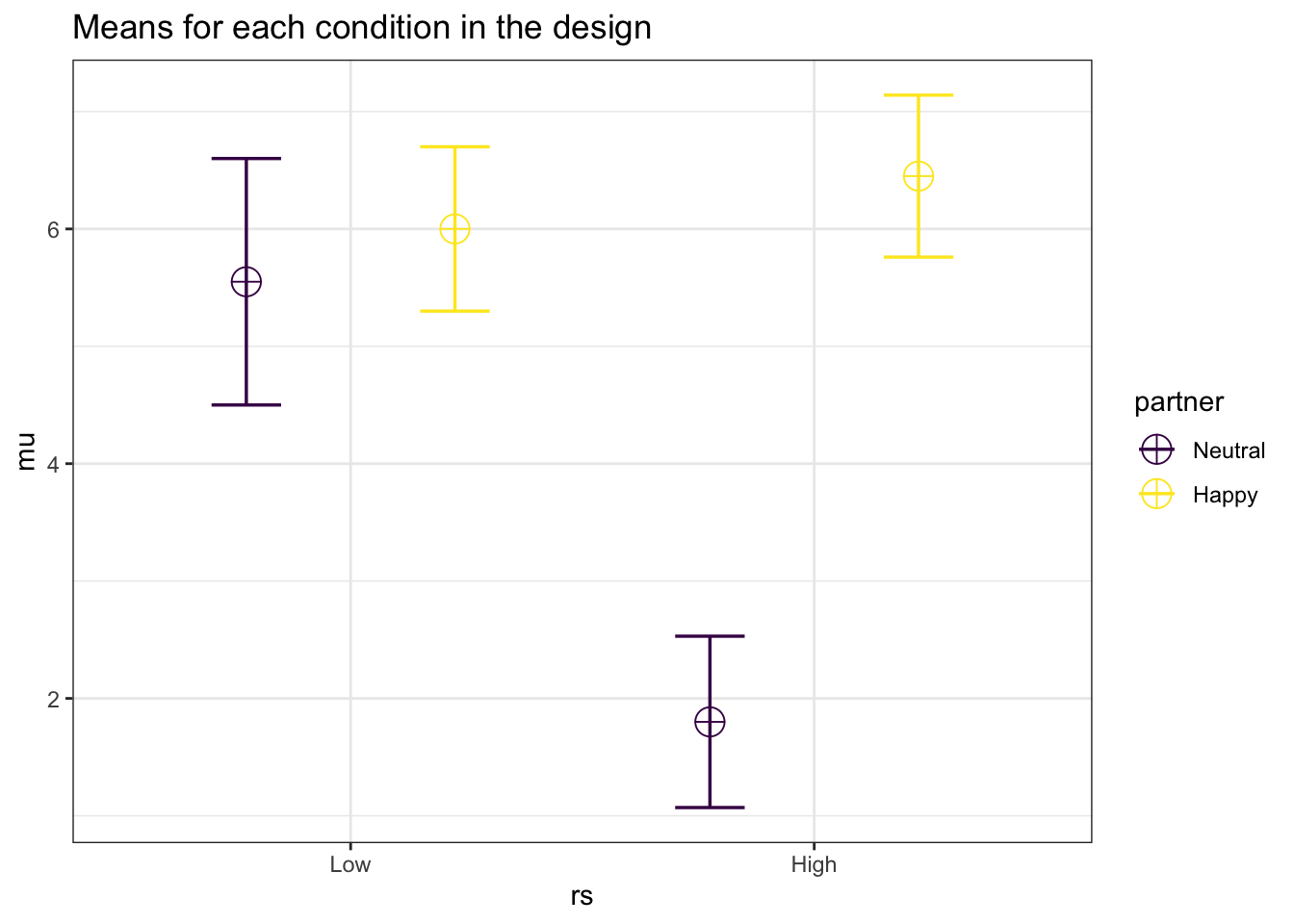

Superpower::ANOVA_power(design_result,
                        alpha_level = 0.05,
                        nsims = 1000, 
                        verbose = FALSE)

Power and Effect sizes for ANOVA tests
                 power effect_size
anova_rs           100      0.5274
anova_partner      100      0.7275
anova_rs:partner   100      0.6439

Power and Effect sizes for pairwise comparisons (t-tests)
                                                 power effect_size
p_rs_Low_partner_Neutral_rs_Low_partner_Happy     35.3      0.5217
p_rs_Low_partner_Neutral_rs_High_partner_Neutral 100.0     -4.2766
p_rs_Low_partner_Neutral_rs_High_partner_Happy    89.2      1.0492
p_rs_Low_partner_Happy_rs_High_partner_Neutral   100.0     -6.0451
p_rs_Low_partner_Happy_rs_High_partner_Happy      52.2      0.6677
p_rs_High_partner_Neutral_rs_High_partner_Happy  100.0      6.7441

Visualization

Use ggplot2 to create nice figures of the main effects and interaction

Main effects

Plotting the main effect of rejection sensitivity

## your code here
library(ggeffects)

model_dev <- lm(liking ~ rs_cat * partner_cat, data = reject_cat)

ggemmeans(model_dev, terms=c("rs_cat")) %>% plot(add.data=TRUE, jitter=.2)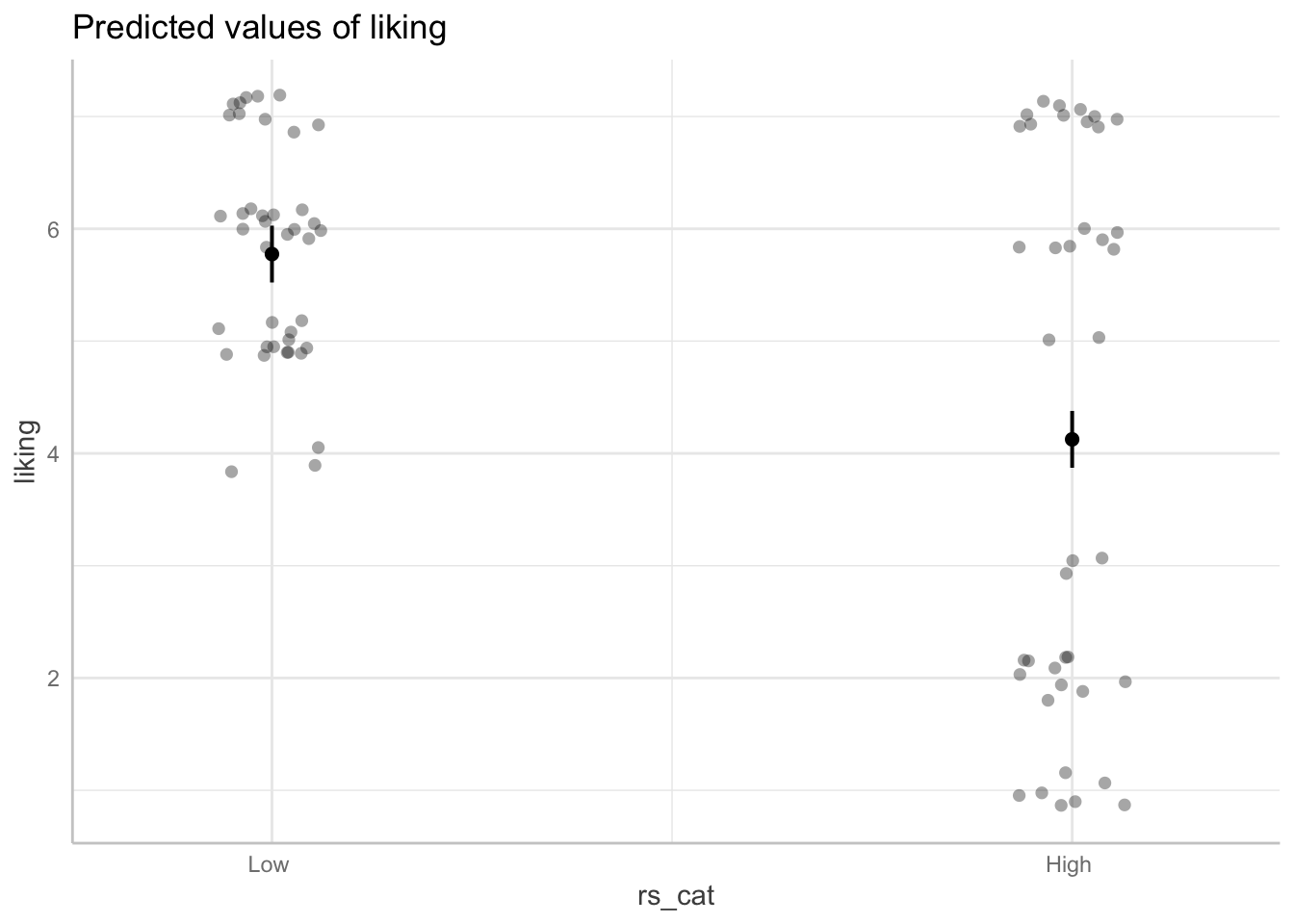

Plotting the main effect of partner’s emotional expression

## your code here

ggemmeans(model_dev, terms=c("partner_cat")) %>% plot(add.data=TRUE, jitter=.2)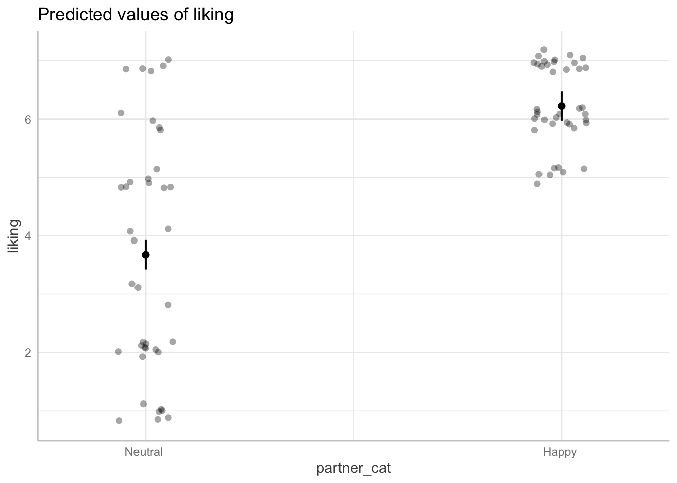

Interaction

Plotting the interaction effect

## your code here


ggemmeans(model_dev, terms=c("rs_cat", "partner_cat")) %>% plot(add.data=TRUE, jitter=.2)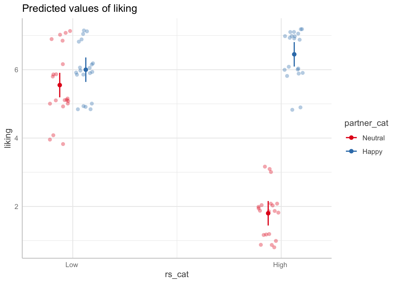

Switch how the interaction is visualized by switching the order of terms

## your code here
ggemmeans(model_dev, terms=c("partner_cat", "rs_cat")) %>% plot(show_data=TRUE, jitter=.2)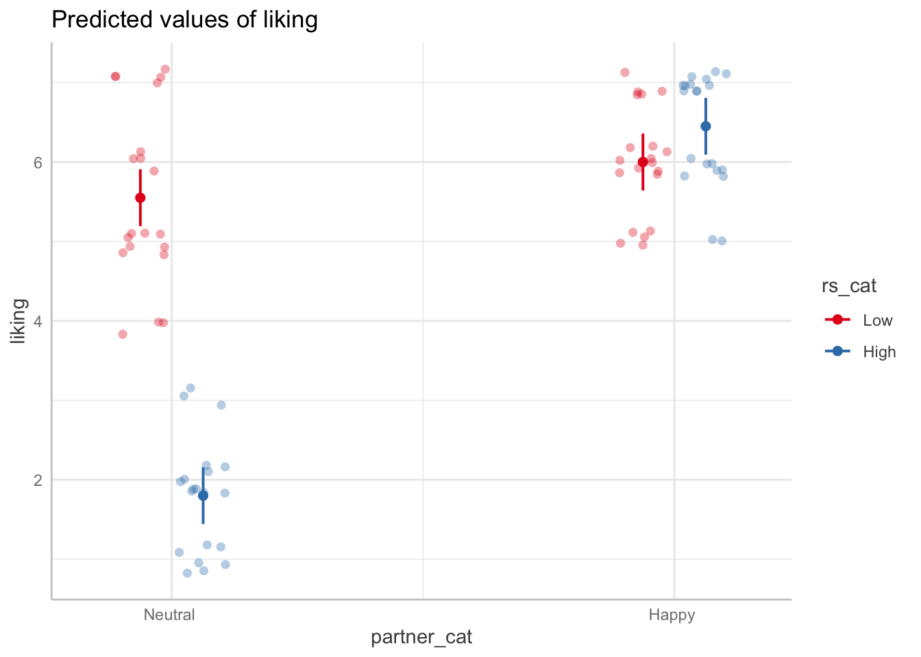

Question: How would you describe in a paper what the significant interaction effect means?

Simple effects

Simple effects are the effect of some factor (e.g., interaction partner’s expression) at each level of another factor (e.g., at high and low RS separately).

Question: Does partner emotion have an effect on perceived liking for people low on rejection sensitivity? For people high on rejection sensitivty?

emmeans::emmeans(model_dev, pairwise~rs_cat*partner_cat) %>%
  joint_tests(by="rs_cat")

rs_cat = Low :
 model term  df1 df2 F.ratio p.value
 partner_cat   1  76   3.134  0.0807

rs_cat = High :
 model term  df1 df2 F.ratio p.value
 partner_cat   1  76 334.686  <.0001

Question: Does rejection sensitivity have an effect on perceived liking when partner shows neutral emotions? When partner shows happy emotions?

## your code here
emmeans::emmeans(model_dev, pairwise~rs_cat*partner_cat) %>%
  joint_tests(by="partner_cat")

partner_cat = Neutral :
 model term df1 df2 F.ratio p.value
 rs_cat       1  76 217.668  <.0001

partner_cat = Happy :
 model term df1 df2 F.ratio p.value
 rs_cat       1  76   3.134  0.0807

Reporting results

Write-up the results from the ANOVA analysis in APA style. Focus on one of the simple effect directions from above (they are equivalent so pick one that makes the most sense)

aov_model <- aov(model_dev)
report(aov_model)

The ANOVA (formula: liking ~ rs_cat * partner_cat) suggests that:

  - The main effect of rs_cat is statistically significant and large (F(1, 76) =
84.28, p < .001; Eta2 (partial) = 0.53, 95% CI [0.40, 1.00])
  - The main effect of partner_cat is statistically significant and large (F(1,
76) = 201.30, p < .001; Eta2 (partial) = 0.73, 95% CI [0.64, 1.00])
  - The interaction between rs_cat and partner_cat is statistically significant
and large (F(1, 76) = 136.52, p < .001; Eta2 (partial) = 0.64, 95% CI [0.54,
1.00])

Effect sizes were labelled following Field's (2013) recommendations.

Research scenario

Import & inspect the data

Descriptive Statistics

Table of Means

Table of Means

Conduct the Factorial ANOVA

Using Regression: lm()

Recoding

Using Traditional ANOVA: afex

Effect sizes

Power

Visualization

Main effects

Plotting the main effect of rejection sensitivity

Plotting the main effect of partner’s emotional expression

Interaction

Plotting the interaction effect

Simple effects

Reporting results

Using Regression: `lm`()

Using Traditional ANOVA: `afex`